 Spectroscopic bins#
This page shows simple, executable examples of how to build
spectroscopic tomographic redshift bins from a parent distribution
using binny.NZTomography.
Compared with photometric binning, spectroscopic binning usually assumes much smaller redshift uncertainties. As a result, the tomographic bins stay much closer to their ideal boundaries, while still allowing small amounts of broadening or bin mixing when a spectroscopic uncertainty model is included.
The main ideas illustrated are:
building spec-z bins from a parent \(n(z)\),
comparing binning schemes,
changing the number of bins,
varying spectroscopic uncertainty terms,
and inspecting the returned result.
All plotting examples below are executable via .. plot::.
Basic spectroscopic binning#
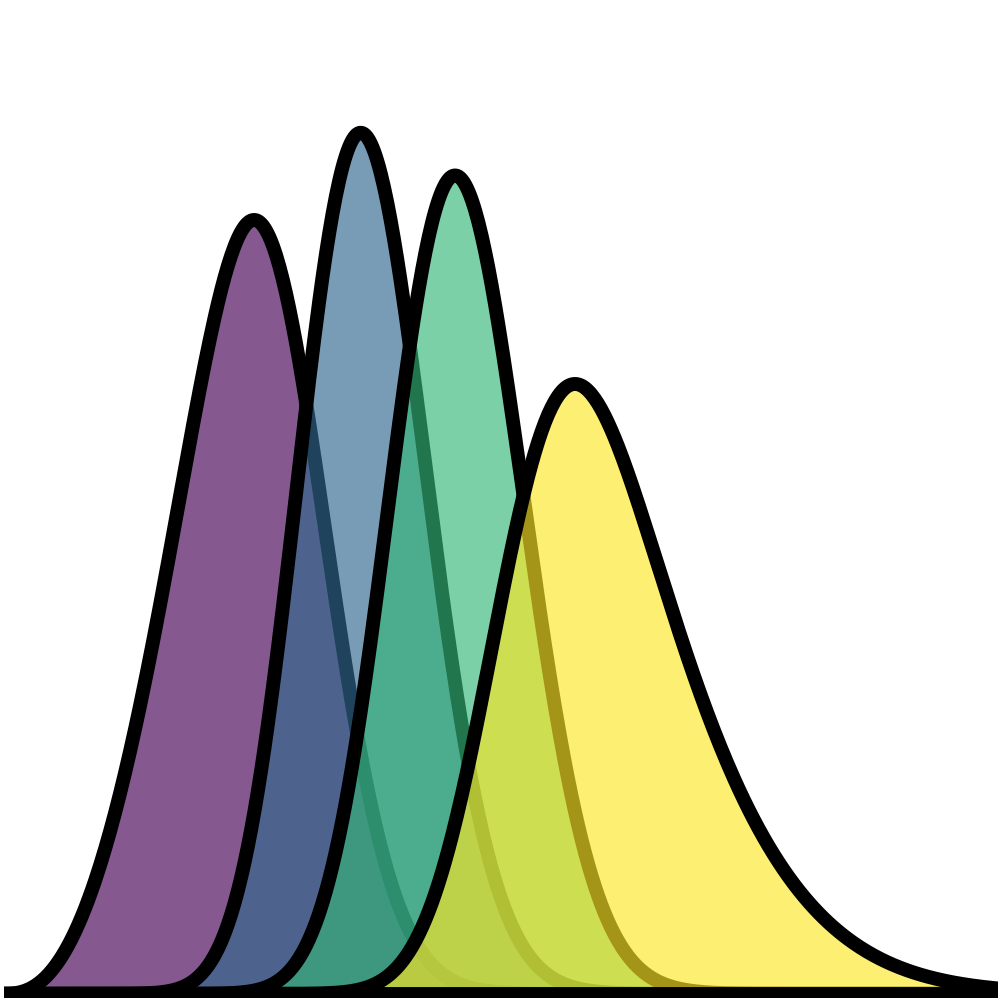
We begin with a simple spectroscopic tomographic setup using a Smail parent distribution, equipopulated binning, and a small spectroscopic scatter term.
import cmasher as cmr
import matplotlib.pyplot as plt
import numpy as np

from binny import NZTomography

def plot_bins(ax, z, bin_dict, title, xmin=0, xmax=1):
    keys = sorted(bin_dict.keys())
    colors = cmr.take_cmap_colors(
        "viridis",
        len(keys),
        cmap_range=(0.0, 1.0),
        return_fmt="hex",
    )

    for i, (color, key) in enumerate(zip(colors, keys, strict=True)):
        curve = np.asarray(bin_dict[key], dtype=float)
        ax.fill_between(
            z,
            0.0,
            curve,
            color=color,
            alpha=0.65,
            linewidth=0.0,
            zorder=10 + i,
        )
        ax.plot(
            z,
            curve,
            color="k",
            linewidth=2.2,
            zorder=20 + i,
        )

    ax.plot(z, np.zeros_like(z), color="k", linewidth=2.2, zorder=1000)
    ax.set_title(title)
    ax.set_xlabel("Redshift $z$")
    ax.set_ylabel(r"Normalized $n_i(z)$")
    ax.set_xlim(xmin, xmax)

tomo = NZTomography()

z = np.linspace(0.0, 1.0, 500)

nz = NZTomography.nz_model(
    "smail",
    z,
    z0=0.12,
    alpha=2.0,
    beta=1.5,
    normalize=True,
)

specz_spec = {
    "kind": "specz",
    "bins": {
        "scheme": "equipopulated",
        "n_bins": 6,
        "range": (0.05, 0.8),
    },
    "normalize_bins": True,
}

specz_result = tomo.build_bins(z=z, nz=nz, tomo_spec=specz_spec)

fig, ax = plt.subplots(figsize=(8.2, 4.8))
plot_bins(
    ax,
    z,
    specz_result.bins,
    title="Spec-z binning: 6 equipopulated bins",
    xmax=0.5
)
plt.tight_layout()
(Source code, png, hires.png, pdf)

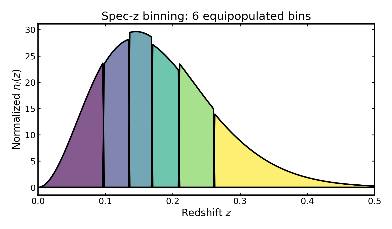
Changing the binning scheme#
As in the photometric case, the choice of binning scheme affects where the tomographic boundaries are placed. Below we compare equidistant and equipopulated spectroscopic bins using the same uncertainty setup.
import cmasher as cmr
import matplotlib.pyplot as plt
import numpy as np

from binny import NZTomography

def plot_bins(ax, z, bin_dict, title, xmin=0, xmax=1):
    keys = sorted(bin_dict.keys())
    colors = cmr.take_cmap_colors(
        "viridis",
        len(keys),
        cmap_range=(0.0, 1.0),
        return_fmt="hex",
    )

    for i, (color, key) in enumerate(zip(colors, keys, strict=True)):
        curve = np.asarray(bin_dict[key], dtype=float)
        ax.fill_between(z, 0.0, curve, color=color, alpha=0.65, linewidth=0.0, zorder=10 + i)
        ax.plot(z, curve, color="k", linewidth=2.2, zorder=20 + i)

    ax.plot(z, np.zeros_like(z), color="k", linewidth=2.2, zorder=1000)
    ax.set_title(title)
    ax.set_xlabel("Redshift $z$")
    ax.set_xlim(xmin, xmax)

tomo = NZTomography()

z = np.linspace(0.0, 1.0, 500)

nz = NZTomography.nz_model(
    "smail",
    z,
    z0=0.12,
    alpha=2.0,
    beta=1.5,
    normalize=True,
)

equidistant_spec = {
    "kind": "specz",
    "bins": {
        "scheme": "equidistant",
        "n_bins": 6,
        "range": (0.05, 0.8),
    },
    "normalize_bins": True,
}

equipopulated_spec = {
    "kind": "specz",
    "bins": {
        "scheme": "equipopulated",
        "n_bins": 6,
        "range": (0.05, 0.8),
    },
    "normalize_bins": True,
}

equidistant_result = tomo.build_bins(
    z=z,
    nz=nz,
    tomo_spec=equidistant_spec,
)
equipopulated_result = tomo.build_bins(
    z=z,
    nz=nz,
    tomo_spec=equipopulated_spec,
)

fig, axes = plt.subplots(1, 2, figsize=(11.0, 4.6), sharey=True)

plot_bins(axes[0], z, equidistant_result.bins, "Equidistant")
axes[0].set_ylabel(r"Normalized $n_i(z)$")

plot_bins(axes[1], z, equipopulated_result.bins, "Equipopulated", xmax=0.5)

plt.tight_layout()
(Source code, png, hires.png, pdf)
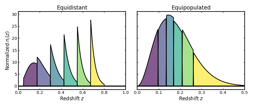
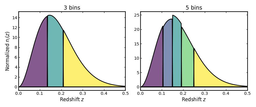
Changing the number of bins#
Increasing n_bins gives a finer tomographic partition.
For spectroscopic binning, the bin edges remain much sharper than in
the photo-z case because the redshift uncertainties are much smaller.
import cmasher as cmr
import matplotlib.pyplot as plt
import numpy as np

from binny import NZTomography

def plot_bins(ax, z, bin_dict, title, xmin=0, xmax=1):
    keys = sorted(bin_dict.keys())
    colors = cmr.take_cmap_colors(
        "viridis",
        len(keys),
        cmap_range=(0.0, 1.0),
        return_fmt="hex",
    )

    for i, (color, key) in enumerate(zip(colors, keys, strict=True)):
        curve = np.asarray(bin_dict[key], dtype=float)
        ax.fill_between(z, 0.0, curve, color=color, alpha=0.65, linewidth=0.0, zorder=10 + i)
        ax.plot(z, curve, color="k", linewidth=2.2, zorder=20 + i)

    ax.plot(z, np.zeros_like(z), color="k", linewidth=2.2, zorder=1000)
    ax.set_title(title)
    ax.set_xlabel("Redshift $z$")
    ax.set_xlim(xmin, xmax)

tomo = NZTomography()

z = np.linspace(0.0, 1.0, 500)

nz = NZTomography.nz_model(
    "smail",
    z,
    z0=0.12,
    alpha=2.0,
    beta=1.5,
    normalize=True,
)

common_bin_uncertainties = {
    "completeness": 1.0,
}

three_bin_spec = {
    "kind": "specz",
    "bins": {
        "scheme": "equipopulated",
        "n_bins": 3,
        "range": (0.05, 0.8),
    },
    "uncertainties": common_bin_uncertainties,
    "normalize_bins": True,
}

five_bin_spec = {
    "kind": "specz",
    "bins": {
        "scheme": "equipopulated",
        "n_bins": 5,
        "range": (0.05, 0.8),
    },
    "uncertainties": common_bin_uncertainties,
    "normalize_bins": True,
}

three_bin_result = tomo.build_bins(z=z, nz=nz, tomo_spec=three_bin_spec)
five_bin_result = tomo.build_bins(z=z, nz=nz, tomo_spec=five_bin_spec)

fig, axes = plt.subplots(1, 2, figsize=(11.0, 4.6))

plot_bins(axes[0], z, three_bin_result.bins, "3 bins", xmax=0.5)
axes[0].set_ylabel(r"Normalized $n_i(z)$")

plot_bins(axes[1], z, five_bin_result.bins, "5 bins", xmax=0.5)

plt.tight_layout()
(Source code, png, hires.png, pdf)
Spectroscopic uncertainties#
The uncertainty parameters can also be used in the spectroscopic case, even though the corresponding values are usually much smaller than in photo-z binning.
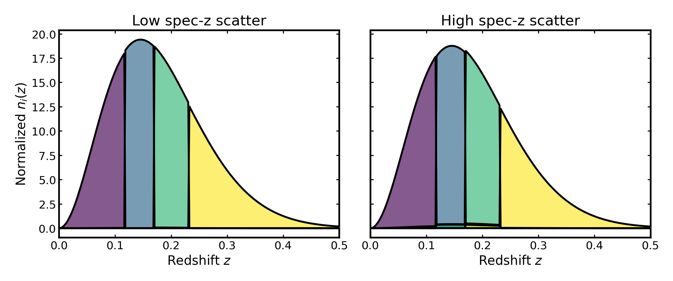
Spectroscopic scatter#
This parameter sets the width of the measurement uncertainty in the
spectroscopic redshift estimate. Although spectroscopic redshifts are typically
very precise, a nonzero specz_scatter slightly broadens the observed
redshift distribution, which smooths the bin edges and introduces a small
overlap between neighboring tomographic bins.
import cmasher as cmr
import matplotlib.pyplot as plt
import numpy as np

from binny import NZTomography

def plot_bins(ax, z, bin_dict, title, xmin=0, xmax=1):
    keys = sorted(bin_dict.keys())
    colors = cmr.take_cmap_colors(
        "viridis",
        len(keys),
        cmap_range=(0.0, 1.0),
        return_fmt="hex",
    )

    for i, (color, key) in enumerate(zip(colors, keys, strict=True)):
        curve = np.asarray(bin_dict[key], dtype=float)
        ax.fill_between(z, 0.0, curve, color=color, alpha=0.65, linewidth=0.0, zorder=10 + i)
        ax.plot(z, curve, color="k", linewidth=2.2, zorder=20 + i)

    ax.plot(z, np.zeros_like(z), color="k", linewidth=2.2, zorder=1000)
    ax.set_title(title)
    ax.set_xlabel("Redshift $z$")
    ax.set_xlim(xmin, xmax)

tomo = NZTomography()

z = np.linspace(0.0, 1.0, 500)

nz = NZTomography.nz_model(
    "smail",
    z,
    z0=0.12,
    alpha=2.0,
    beta=1.5,
    normalize=True,
)

low_scatter_spec = {
    "kind": "specz",
    "bins": {
        "scheme": "equipopulated",
        "n_bins": 4,
    },
    "uncertainties": {
        "completeness": [1.0, 1.0, 1.0, 1.0],
        "specz_scatter": [0.0005, 0.0005, 0.00075, 0.001],
    },
    "normalize_bins": True,
}

high_scatter_spec = {
    "kind": "specz",
    "bins": {
        "scheme": "equipopulated",
        "n_bins": 4,
    },
    "uncertainties": {
        "completeness": [1.0, 1.0, 1.0, 1.0],
        "specz_scatter": [0.003, 0.003, 0.004, 0.005],
    },
    "normalize_bins": True,
}

low_scatter = tomo.build_bins(z=z, nz=nz, tomo_spec=low_scatter_spec)
high_scatter = tomo.build_bins(
    z=z,
    nz=nz,
    tomo_spec=high_scatter_spec,
)

fig, axes = plt.subplots(1, 2, figsize=(11.0, 4.6), sharey=True)

plot_bins(axes[0], z, low_scatter.bins, "Low spec-z scatter", xmax=0.5)
axes[0].set_ylabel(r"Normalized $n_i(z)$")

plot_bins(axes[1], z, high_scatter.bins, "High spec-z scatter", xmax=0.5)

plt.tight_layout()
(Source code, png, hires.png, pdf)

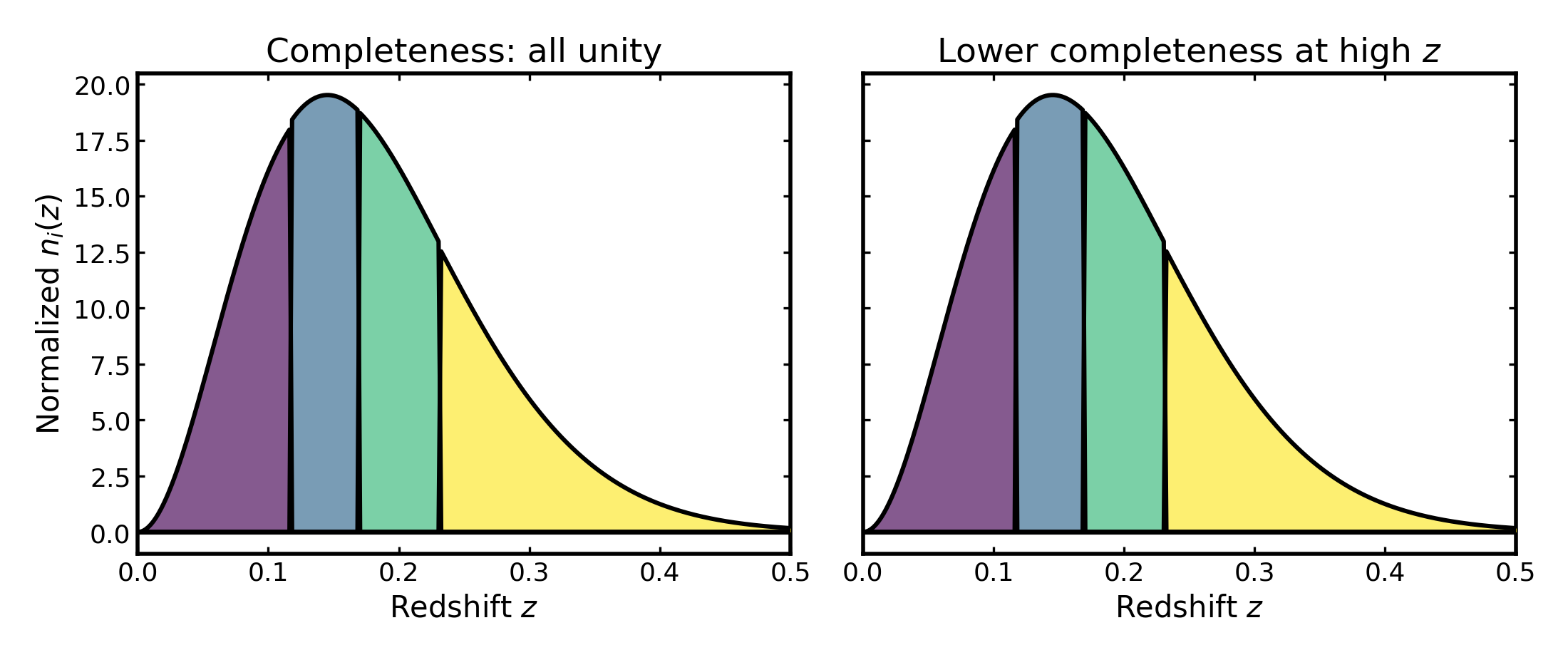
Completeness#
This parameter gives the fraction of galaxies in each bin that are
successfully observed and assigned a reliable spectroscopic redshift.
A value of 1 means that all galaxies in the bin are retained, while
lower values reduce the amplitude of the corresponding tomographic
distribution to reflect incomplete sampling.
import cmasher as cmr
import matplotlib.pyplot as plt
import numpy as np

from binny import NZTomography

def plot_bins(ax, z, bin_dict, title, xmin=0, xmax=1):
    keys = sorted(bin_dict.keys())
    colors = cmr.take_cmap_colors(
        "viridis",
        len(keys),
        cmap_range=(0.0, 1.0),
        return_fmt="hex",
    )

    for i, (color, key) in enumerate(zip(colors, keys, strict=True)):
        curve = np.asarray(bin_dict[key], dtype=float)
        ax.fill_between(z, 0.0, curve, color=color, alpha=0.65, linewidth=0.0, zorder=10 + i)
        ax.plot(z, curve, color="k", linewidth=2.2, zorder=20 + i)

    ax.plot(z, np.zeros_like(z), color="k", linewidth=2.2, zorder=1000)
    ax.set_title(title)
    ax.set_xlabel("Redshift $z$")
    ax.set_xlim(xmin, xmax)

tomo = NZTomography()

z = np.linspace(0.0, 1.0, 500)

nz = NZTomography.nz_model(
    "smail",
    z,
    z0=0.12,
    alpha=2.0,
    beta=1.5,
    normalize=True,
)

complete_spec = {
    "kind": "specz",
    "bins": {
        "scheme": "equipopulated",
        "n_bins": 4,
    },
    "uncertainties": {
        "completeness": 1,  # all bins have full completeness
    },
    "normalize_bins": True,
}

reduced_completeness_spec = {
    "kind": "specz",
    "bins": {
        "scheme": "equipopulated",
        "n_bins": 4,
    },
    "uncertainties": {
        "completeness": [1.0, 0.9, 0.75, 0.7],
    },
    "normalize_bins": True,
}

complete_result = tomo.build_bins(z=z, nz=nz, tomo_spec=complete_spec)
reduced_result = tomo.build_bins(
    z=z,
    nz=nz,
    tomo_spec=reduced_completeness_spec,
)

fig, axes = plt.subplots(1, 2, figsize=(11.0, 4.6), sharey=True)

plot_bins(
   axes[0],
   z,
   complete_result.bins,
   "Completeness: all unity",
   xmax=0.5
)
axes[0].set_ylabel(r"Normalized $n_i(z)$")

plot_bins(
   axes[1],
   z,
   reduced_result.bins,
   "Lower completeness at high $z$",
   xmax=0.5
)

plt.tight_layout()
(Source code, png, hires.png, pdf)
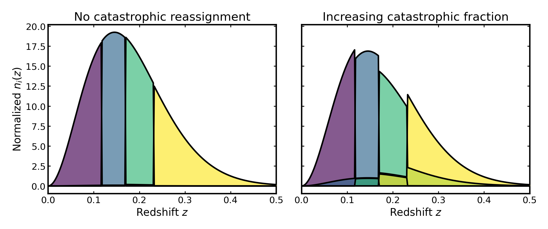
Catastrophic misassignment#
This parameter sets the fraction of galaxies whose spectroscopic
redshift assignment fails catastrophically. These galaxies are then
redistributed into other bins according to the chosen leakage model.
Increasing catastrophic_frac therefore increases mixing between
otherwise well-separated tomographic bins.
import cmasher as cmr
import matplotlib.pyplot as plt
import numpy as np

from binny import NZTomography

def plot_bins(ax, z, bin_dict, title, xmin=0, xmax=1):
    keys = sorted(bin_dict.keys())
    colors = cmr.take_cmap_colors(
        "viridis",
        len(keys),
        cmap_range=(0.0, 1.0),
        return_fmt="hex",
    )

    for i, (color, key) in enumerate(zip(colors, keys, strict=True)):
        curve = np.asarray(bin_dict[key], dtype=float)
        ax.fill_between(z, 0.0, curve, color=color, alpha=0.65, linewidth=0.0, zorder=10 + i)
        ax.plot(z, curve, color="k", linewidth=2.2, zorder=20 + i)

    ax.plot(z, np.zeros_like(z), color="k", linewidth=2.2, zorder=1000)
    ax.set_title(title)
    ax.set_xlabel("Redshift $z$")
    ax.set_xlim(xmin, xmax)

tomo = NZTomography()

z = np.linspace(0.0, 1.0, 500)

nz = NZTomography.nz_model(
    "smail",
    z,
    z0=0.12,
    alpha=2.0,
    beta=1.5,
    normalize=True,
)

no_catastrophic_spec = {
    "kind": "specz",
    "bins": {
        "scheme": "equipopulated",
        "n_bins": 4,
    },
    "uncertainties": {
        "completeness": 1,
        "catastrophic_frac": [0.0, 0.0, 0.0, 0.0],
        "specz_scatter": [0.001, 0.001, 0.0015, 0.002],
    },
    "normalize_bins": True,
}

catastrophic_spec = {
    "kind": "specz",
    "bins": {
        "scheme": "equipopulated",
        "n_bins": 4,
    },
    "uncertainties": {
        "completeness": 1,
        "catastrophic_frac": [0.05, 0.1, 0.15, 0.2],
        "leakage_model": "neighbor",
        "specz_scatter": [0.001, 0.001, 0.0015, 0.002],
    },
    "normalize_bins": True,
}

no_catastrophic_result = tomo.build_bins(
    z=z,
    nz=nz,
    tomo_spec=no_catastrophic_spec,
)
catastrophic_result = tomo.build_bins(
    z=z,
    nz=nz,
    tomo_spec=catastrophic_spec,
)

fig, axes = plt.subplots(1, 2, figsize=(11.0, 4.6), sharey=True)

plot_bins(
    axes[0],
    z,
    no_catastrophic_result.bins,
    "No catastrophic reassignment",
    xmax=0.5
)
axes[0].set_ylabel(r"Normalized $n_i(z)$")

plot_bins(
    axes[1],
    z,
    catastrophic_result.bins,
    "Increasing catastrophic fraction",
    xmax=0.5
)

plt.tight_layout()
(Source code, png, hires.png, pdf)

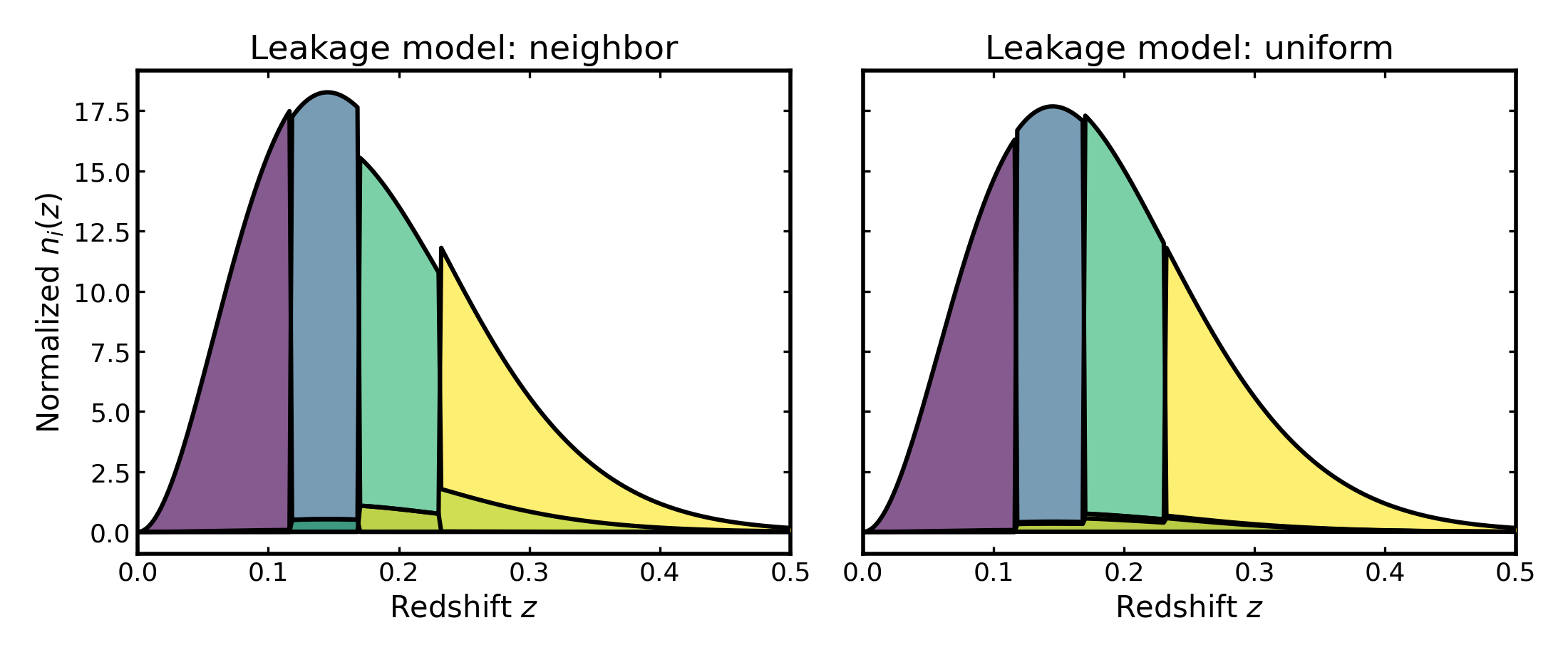
Leakage model#
This parameter defines how galaxies affected by catastrophic redshift
failures are redistributed across bins. The neighbor model moves
misassigned galaxies mainly into adjacent bins, while uniform
spreads them across all bins with equal probability.
import cmasher as cmr
import matplotlib.pyplot as plt
import numpy as np

from binny import NZTomography

def plot_bins(ax, z, bin_dict, title, xmin=0, xmax=1):
    keys = sorted(bin_dict.keys())
    colors = cmr.take_cmap_colors(
        "viridis",
        len(keys),
        cmap_range=(0.0, 1.0),
        return_fmt="hex",
    )

    for i, (color, key) in enumerate(zip(colors, keys, strict=True)):
        curve = np.asarray(bin_dict[key], dtype=float)
        ax.fill_between(z, 0.0, curve, color=color, alpha=0.65, linewidth=0.0, zorder=10 + i)
        ax.plot(z, curve, color="k", linewidth=2.2, zorder=20 + i)

    ax.plot(z, np.zeros_like(z), color="k", linewidth=2.2, zorder=1000)
    ax.set_title(title)
    ax.set_xlabel("Redshift $z$")
    ax.set_xlim(xmin, xmax)

tomo = NZTomography()

z = np.linspace(0.0, 1.0, 500)

nz = NZTomography.nz_model(
    "smail",
    z,
    z0=0.12,
    alpha=2.0,
    beta=1.5,
    normalize=True,
)

neighbor_spec = {
    "kind": "specz",
    "bins": {
        "scheme": "equipopulated",
        "n_bins": 4,
    },
    "uncertainties": {
        "completeness": [1.0, 1.0, 1.0, 1.0],
        "catastrophic_frac": [0.0, 0.05, 0.1, 0.15],
        "leakage_model": "neighbor",
        "specz_scatter": [0.001, 0.001, 0.0015, 0.002],
    },
    "normalize_bins": True,
}

uniform_spec = {
    "kind": "specz",
    "bins": {
        "scheme": "equipopulated",
        "n_bins": 4,
    },
    "uncertainties": {
        "completeness": [1.0, 1.0, 1.0, 1.0],
        "catastrophic_frac": [0.0, 0.05, 0.1, 0.15],
        "leakage_model": "uniform",
        "specz_scatter": [0.001, 0.001, 0.0015, 0.002],
    },
    "normalize_bins": True,
}

neighbor_result = tomo.build_bins(z=z, nz=nz, tomo_spec=neighbor_spec)
uniform_result = tomo.build_bins(z=z, nz=nz, tomo_spec=uniform_spec)

fig, axes = plt.subplots(1, 2, figsize=(11.0, 4.6), sharey=True)

plot_bins(axes[0], z, neighbor_result.bins, "Leakage model: neighbor", xmax=0.5)
axes[0].set_ylabel(r"Normalized $n_i(z)$")

plot_bins(axes[1], z, uniform_result.bins, "Leakage model: uniform", xmax=0.5)

plt.tight_layout()
(Source code, png, hires.png, pdf)

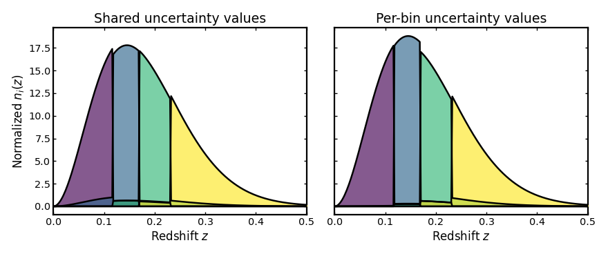
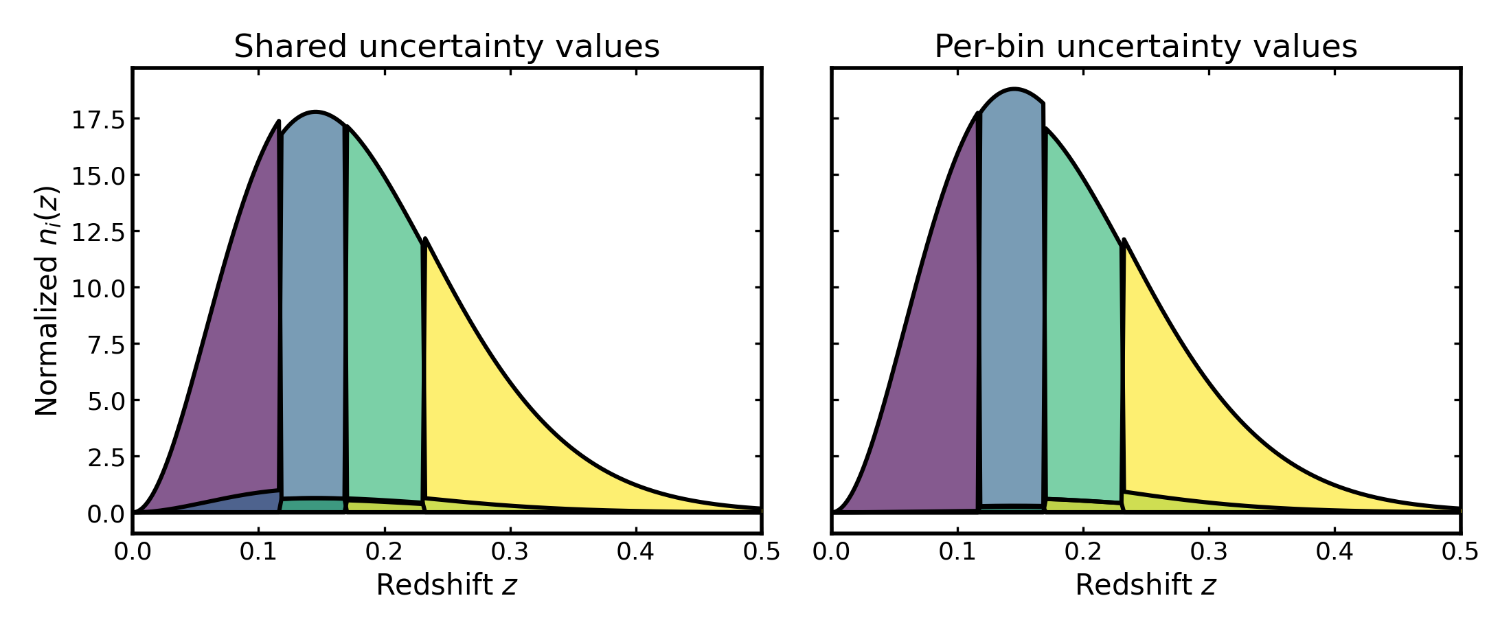
Per-bin versus shared uncertainties#
Spectroscopic uncertainty parameters can also be supplied either as a single value applied across all tomographic bins or as a list with one value per bin. This is useful when comparing a simplified global model with a more realistic bin-dependent one.
The example below compares a shared spectroscopic scatter and completeness model with a per-bin version of the same setup.
import cmasher as cmr
import matplotlib.pyplot as plt
import numpy as np

from binny import NZTomography

def plot_bins(ax, z, bin_dict, title, xmin=0, xmax=1):
    keys = sorted(bin_dict.keys())
    colors = cmr.take_cmap_colors(
        "viridis",
        len(keys),
        cmap_range=(0.0, 1.0),
        return_fmt="hex",
    )

    for i, (color, key) in enumerate(zip(colors, keys, strict=True)):
        curve = np.asarray(bin_dict[key], dtype=float)
        ax.fill_between(
            z,
            0.0,
            curve,
            color=color,
            alpha=0.65,
            linewidth=0.0,
            zorder=10 + i,
        )
        ax.plot(
            z,
            curve,
            color="k",
            linewidth=2.2,
            zorder=20 + i,
        )

    ax.plot(z, np.zeros_like(z), color="k", linewidth=2.2, zorder=1000)
    ax.set_title(title)
    ax.set_xlabel("Redshift $z$")
    ax.set_xlim(xmin, xmax)

tomo = NZTomography()

z = np.linspace(0.0, 1.0, 500)

nz = NZTomography.nz_model(
    "smail",
    z,
    z0=0.12,
    alpha=2.0,
    beta=1.5,
    normalize=True,
)

shared_uncertainty_spec = {
    "kind": "specz",
    "bins": {
        "scheme": "equipopulated",
        "n_bins": 4,
    },
    "uncertainties": {
        "completeness": 0.95,
        "catastrophic_frac": 0.05,
        "leakage_model": "neighbor",
        "specz_scatter": 0.0015,
    },
    "normalize_bins": True,
}

per_bin_uncertainty_spec = {
    "kind": "specz",
    "bins": {
        "scheme": "equipopulated",
        "n_bins": 4,
    },
    "uncertainties": {
        "completeness": [1.0, 0.98, 0.92, 0.85],
        "catastrophic_frac": [0.0, 0.02, 0.05, 0.08],
        "leakage_model": "neighbor",
        "specz_scatter": [0.0008, 0.001, 0.0015, 0.002],
    },
    "normalize_bins": True,
}

shared_result = tomo.build_bins(
    z=z,
    nz=nz,
    tomo_spec=shared_uncertainty_spec,
)
per_bin_result = tomo.build_bins(
    z=z,
    nz=nz,
    tomo_spec=per_bin_uncertainty_spec,
)

fig, axes = plt.subplots(1, 2, figsize=(11.0, 4.6), sharey=True)

plot_bins(axes[0], z, shared_result.bins, "Shared uncertainty values", xmax=0.5)
axes[0].set_ylabel(r"Normalized $n_i(z)$")

plot_bins(axes[1], z, per_bin_result.bins, "Per-bin uncertainty values", xmax=0.5)

plt.tight_layout()
(Source code, png, hires.png, pdf)

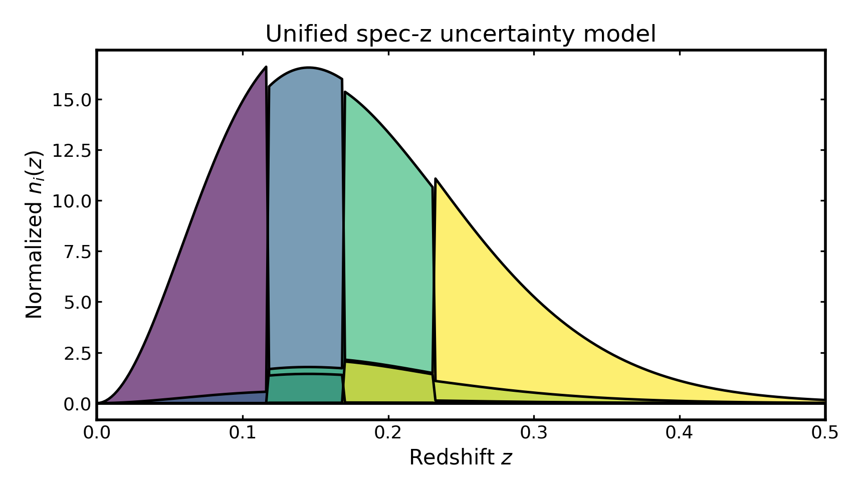
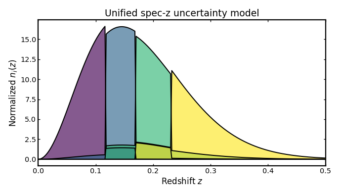
Unified spectroscopic uncertainty model#
This example combines several spectroscopic uncertainty terms in one setup: per-bin completeness, catastrophic redshift failures, a leakage model, and small spectroscopic scatter. In practice, this is often a more realistic configuration than varying one ingredient at a time, because real spectroscopic samples can be affected by several effects simultaneously.
The example below uses per-bin values for completeness,
catastrophic_frac, and specz_scatter.
import cmasher as cmr
import matplotlib.pyplot as plt
import numpy as np

from binny import NZTomography

def plot_bins(ax, z, bin_dict, title, xmin=0, xmax=1):
    keys = sorted(bin_dict.keys())
    colors = cmr.take_cmap_colors(
        "viridis",
        len(keys),
        cmap_range=(0.0, 1.0),
        return_fmt="hex",
    )

    for i, (color, key) in enumerate(zip(colors, keys, strict=True)):
        curve = np.asarray(bin_dict[key], dtype=float)
        ax.fill_between(
            z,
            0.0,
            curve,
            color=color,
            alpha=0.65,
            linewidth=0.0,
            zorder=10 + i,
        )
        ax.plot(
            z,
            curve,
            color="k",
            linewidth=1.8,
            zorder=20 + i,
        )

    ax.plot(z, np.zeros_like(z), color="k", linewidth=1.8, zorder=1000)
    ax.set_title(title)
    ax.set_xlabel("Redshift $z$")
    ax.set_ylabel(r"Normalized $n_i(z)$")
    ax.set_xlim(xmin, xmax)

tomo = NZTomography()

z = np.linspace(0.0, 1.0, 500)

nz = NZTomography.nz_model(
    "smail",
    z,
    z0=0.12,
    alpha=2.0,
    beta=1.5,
    normalize=True,
)

unified_uncertainty_spec = {
    "kind": "specz",
    "bins": {
        "scheme": "equipopulated",
        "n_bins": 4,
    },
    "uncertainties": {
        "completeness": [1.0, 0.97, 0.92, 0.85],
        "catastrophic_frac": [0.0, 0.02, 0.05, 0.08],
        "leakage_model": "neighbor",
        "specz_scatter": [0.008, 0.01, 0.015, 0.052],
    },
    "normalize_bins": True,
}

unified_result = tomo.build_bins(
    z=z,
    nz=nz,
    tomo_spec=unified_uncertainty_spec,
)

fig, ax = plt.subplots(figsize=(8.6, 4.9))
plot_bins(
    ax,
    z,
    unified_result.bins,
    title="Unified spec-z uncertainty model",
    xmax=0.5
)
plt.tight_layout()
(Source code, png, hires.png, pdf)
Inspecting the returned bins#
The object returned by binny.NZTomography.build_bins() stores the
parent distribution, the resolved specification, and the tomographic bin
curves. You can inspect these contents directly before using the result
elsewhere.
import numpy as np

from binny import NZTomography

tomo = NZTomography()

z = np.linspace(0.0, 1.0, 500)

nz = NZTomography.nz_model(
    "smail",
    z,
    z0=0.12,
    alpha=2.0,
    beta=1.5,
    normalize=True,
)

specz_spec = {
    "kind": "specz",
    "bins": {
        "scheme": "equipopulated",
        "n_bins": 4,
    },
    "uncertainties": {
        "completeness": [1.0, 0.95, 0.9, 0.85],
        "catastrophic_frac": [0.0, 0.05, 0.1, 0.15],
        "leakage_model": "neighbor",
        "specz_scatter": [0.001, 0.001, 0.0015, 0.002],
    },
    "normalize_bins": True,
}

specz_result = tomo.build_bins(z=z, nz=nz, tomo_spec=specz_spec)

print("Bin keys:")
print(list(specz_result.bins.keys()))
print()
print("Parent shape:", specz_result.nz.shape)
first_key = sorted(specz_result.bins.keys())[0]
print("First bin shape:", specz_result.bins[first_key].shape)
print("Resolved kind:", specz_result.spec["kind"])
print("Resolved scheme:", specz_result.spec["bins"]["scheme"])
print("Resolved n_bins:", specz_result.spec["bins"]["n_bins"])
Notes#
These examples use
binny.NZTomography.build_bins()with a compacttomo_specmapping.When building bins from arrays, pass all three pieces explicitly:
z,nz, andtomo_spec.In the spectroscopic case, the supported uncertainty terms follow the spec-z schema, such as
completeness,catastrophic_frac,leakage_model, andspecz_scatter.The plotting style here uses filled tomographic curves with black outlines, matching the photometric examples and broader Binny visual style.
The scheme names used in the API are
equidistantandequipopulated.