 Photometric bins#
This page shows simple, executable examples of how to build
photometric tomographic redshift bins from a parent distribution
using binny.NZTomography.
In contrast to spectroscopic binning, photometric binning requires a photo-z uncertainty model. This page introduces both the basic photo-z workflow and the effect of individual uncertainty terms on the resulting tomographic bins.
The main ideas illustrated are:
building photo-z bins from a parent \(n(z)\),
comparing binning schemes,
changing the number of bins,
varying individual photo-z uncertainty terms,
and combining all uncertainty ingredients in one setup.
All plotting examples below are executable via .. plot::.
Basic photometric binning#
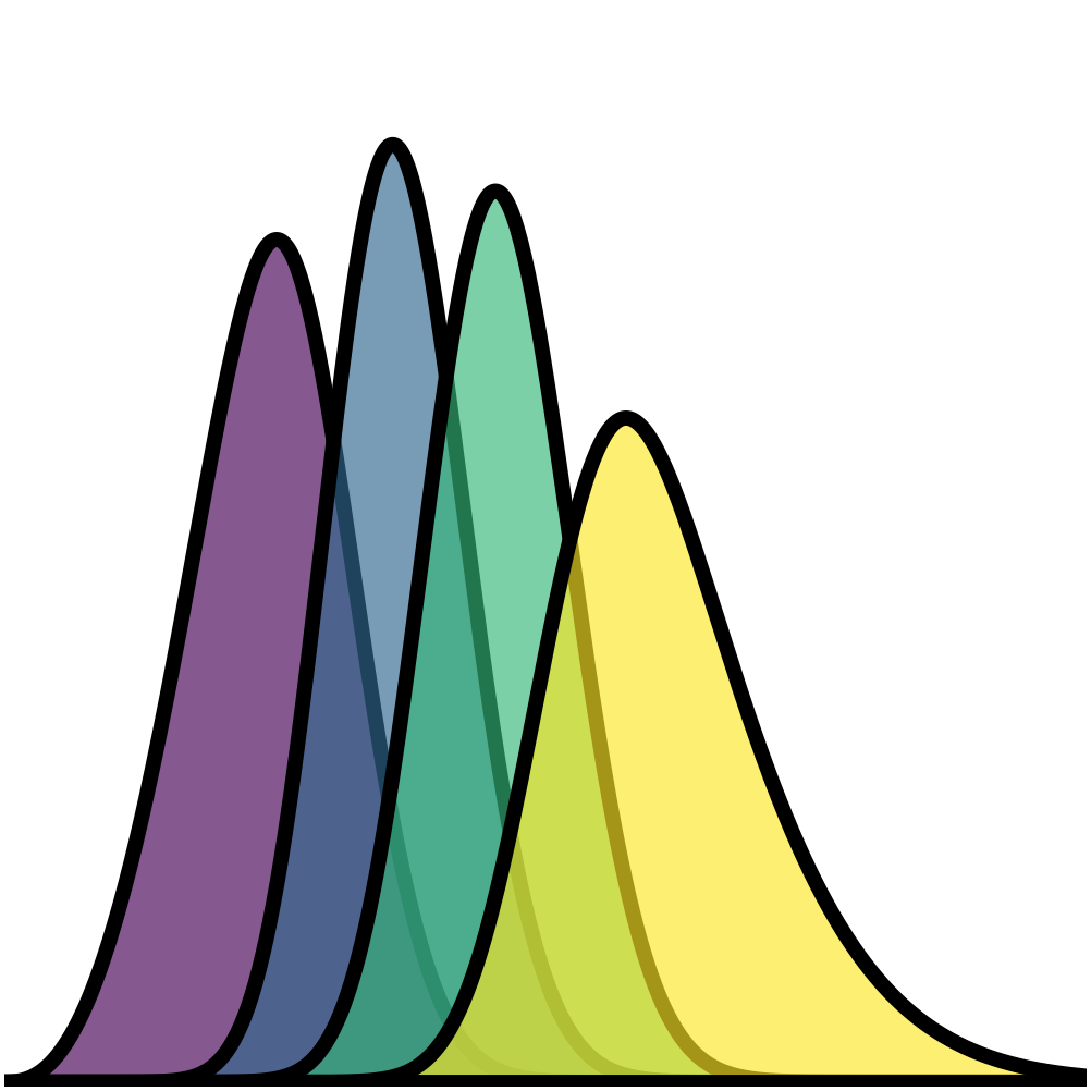
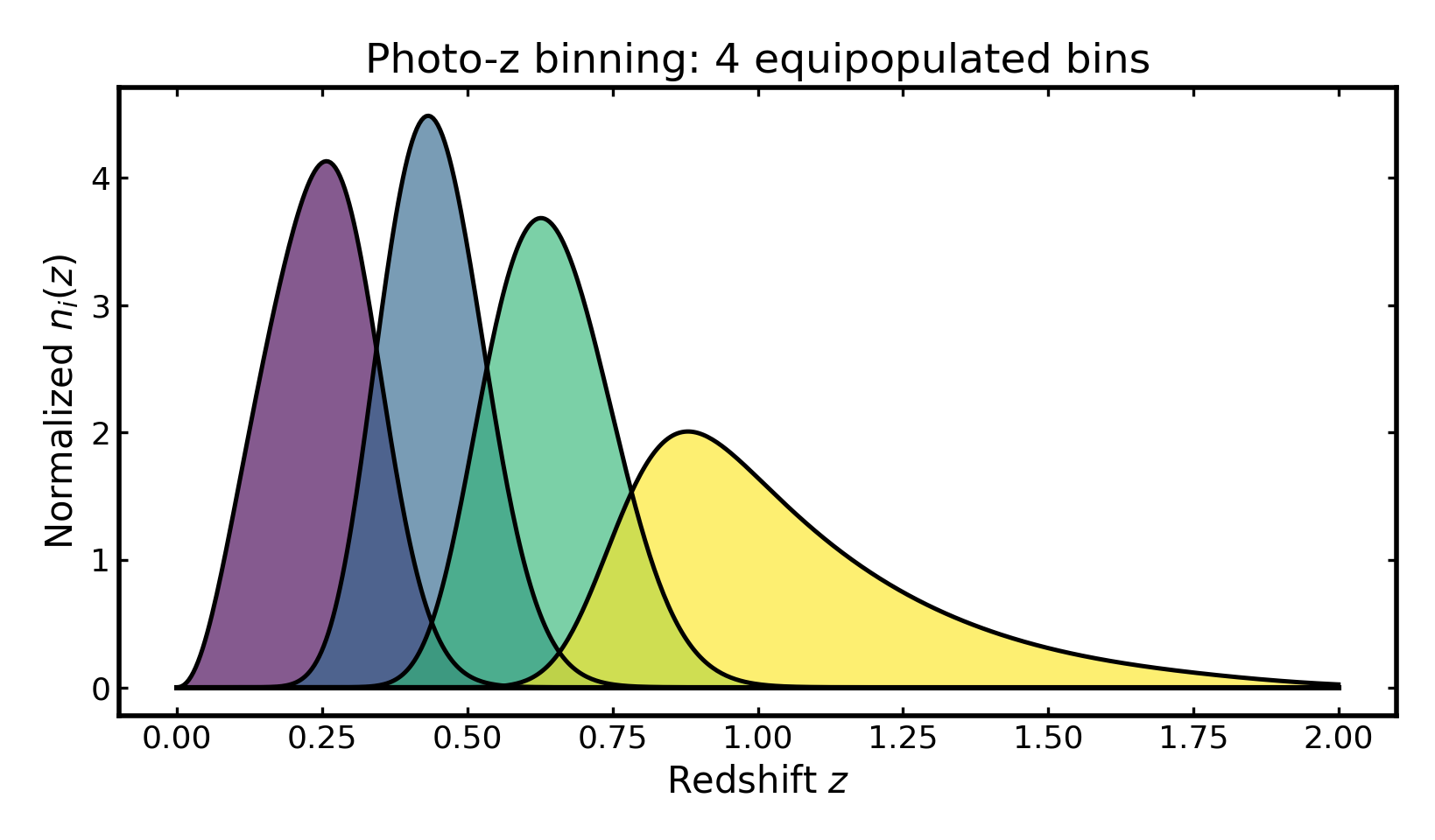
We first construct a simple photo-z tomographic setup using a Smail parent distribution, equipopulated binning, and a single scalar scatter term.
import cmasher as cmr
import matplotlib.pyplot as plt
import numpy as np

from binny import NZTomography

def plot_bins(ax, z, bin_dict, title, cmap="viridis", cmap_range=(0.0, 1.0)):
    keys = sorted(bin_dict.keys())
    colors = cmr.take_cmap_colors(
        cmap,
        len(keys),
        cmap_range=cmap_range,
        return_fmt="hex",
    )

    for i, (color, key) in enumerate(zip(colors, keys, strict=True)):
        curve = np.asarray(bin_dict[key], dtype=float)
        ax.fill_between(
            z,
            0.0,
            curve,
            color=color,
            alpha=0.65,
            linewidth=0.0,
            zorder=10 + i,
        )
        ax.plot(
            z,
            curve,
            color="k",
            linewidth=1.8,
            zorder=20 + i,
        )

    ax.plot(z, np.zeros_like(z), color="k", linewidth=2.2, zorder=1000)
    ax.set_title(title)
    ax.set_xlabel("Redshift $z$")
    ax.set_ylabel(r"Normalized $n_i(z)$")

tomo = NZTomography()

z = np.linspace(0.0, 2.0, 500)

nz = NZTomography.nz_model(
    "smail",
    z,
    z0=0.2,
    alpha=2.0,
    beta=1.0,
    normalize=True,
)

photoz_spec = {
    "kind": "photoz",
    "bins": {
        "scheme": "equipopulated",
        "n_bins": 4,
    },
    "uncertainties": {
        "scatter_scale": 0.05,
    },
    "normalize_bins": True,
}

photoz_result = tomo.build_bins(z=z, nz=nz, tomo_spec=photoz_spec)

fig, ax = plt.subplots(figsize=(8.2, 4.8))
plot_bins(
    ax,
    z,
    photoz_result.bins,
    title="Photo-z binning: 4 equipopulated bins",
)
plt.tight_layout()
(Source code, png, hires.png, pdf)
Changing the binning scheme#
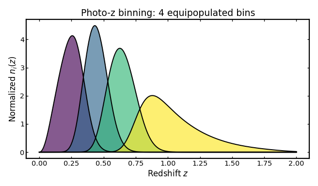
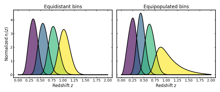
Tomographic bins can be defined in different ways. The two most common approaches are equidistant bins, where the redshift interval is split uniformly, and equipopulated bins, where each bin contains roughly the same number of galaxies. The example below compares these two strategies using the same parent distribution and photo-z uncertainty model.
import cmasher as cmr
import matplotlib.pyplot as plt
import numpy as np

from binny import NZTomography

def plot_bins(ax, z, bin_dict, title, cmap="viridis", cmap_range=(0.0, 1.0)):
    keys = sorted(bin_dict.keys())
    colors = cmr.take_cmap_colors(
        cmap,
        len(keys),
        cmap_range=cmap_range,
        return_fmt="hex",
    )

    for i, (color, key) in enumerate(zip(colors, keys, strict=True)):
        curve = np.asarray(bin_dict[key], dtype=float)
        ax.fill_between(z, 0.0, curve, color=color, alpha=0.65, linewidth=0.0, zorder=10 + i)
        ax.plot(z, curve, color="k", linewidth=2.2, zorder=20 + i)

    ax.plot(z, np.zeros_like(z), color="k", linewidth=2.2, zorder=1000)
    ax.set_title(title)
    ax.set_xlabel("Redshift $z$")

tomo = NZTomography()

z = np.linspace(0.0, 2.0, 500)

nz = NZTomography.nz_model(
    "smail",
    z,
    z0=0.2,
    alpha=2.0,
    beta=1.0,
    normalize=True,
)

common_uncertainties = {"scatter_scale": 0.05}

equidistant_spec = {
    "kind": "photoz",
    "bins": {
    "scheme": "equidistant",
    "n_bins": 4,
    "range": (0.2, 1.2),  # define a custom redshift range for the equidistant bins
},
    "uncertainties": common_uncertainties,
    "normalize_bins": True,
}

equipopulated_spec = {
    "kind": "photoz",
    "bins": {"scheme": "equipopulated", "n_bins": 4},
    "uncertainties": common_uncertainties,
    "normalize_bins": True,
}

equidistant_result = tomo.build_bins(z=z, nz=nz, tomo_spec=equidistant_spec)
equipopulated_result = tomo.build_bins(z=z, nz=nz, tomo_spec=equipopulated_spec)

fig, axes = plt.subplots(1, 2, figsize=(11.0, 4.6), sharey=True)

plot_bins(axes[0], z, equidistant_result.bins, "Equidistant bins")
axes[0].set_ylabel(r"Normalized $n_i(z)$")

plot_bins(axes[1], z, equipopulated_result.bins, "Equipopulated bins")

plt.tight_layout()
(Source code, png, hires.png, pdf)
Changing the number of bins#
The number of tomographic bins is another important design choice in cosmological analyses. Increasing the number of bins improves redshift resolution but also increases noise and the number of cross-correlations. The example below compares two setups with different bin counts while keeping the parent distribution and uncertainty model fixed.
import cmasher as cmr
import matplotlib.pyplot as plt
import numpy as np

from binny import NZTomography

def plot_bins(ax, z, bin_dict, title, cmap="viridis", cmap_range=(0.0, 1.0)):
    keys = sorted(bin_dict.keys())
    colors = cmr.take_cmap_colors(
        cmap,
        len(keys),
        cmap_range=cmap_range,
        return_fmt="hex",
    )

    for i, (color, key) in enumerate(zip(colors, keys, strict=True)):
        curve = np.asarray(bin_dict[key], dtype=float)
        ax.fill_between(z, 0.0, curve, color=color, alpha=0.65, linewidth=0.0, zorder=10 + i)
        ax.plot(z, curve, color="k", linewidth=2.2, zorder=20 + i)

    ax.plot(z, np.zeros_like(z), color="k", linewidth=2.2, zorder=1000)
    ax.set_title(title)
    ax.set_xlabel("Redshift $z$")

tomo = NZTomography()

z = np.linspace(0.0, 2.0, 500)

nz = NZTomography.nz_model(
    "smail",
    z,
    z0=0.2,
    alpha=2.0,
    beta=1.0,
    normalize=True,
)

common_uncertainties = {"scatter_scale": 0.05}

three_bins_spec = {
    "kind": "photoz",
    "bins": {"scheme": "equipopulated", "n_bins": 3},
    "uncertainties": common_uncertainties,
    "normalize_bins": True,
}

five_bins_spec = {
    "kind": "photoz",
    "bins": {"scheme": "equipopulated", "n_bins": 5},
    "uncertainties": common_uncertainties,
    "normalize_bins": True,
}

three_bin_result = tomo.build_bins(z=z, nz=nz, tomo_spec=three_bins_spec)
five_bin_result = tomo.build_bins(z=z, nz=nz, tomo_spec=five_bins_spec)

fig, axes = plt.subplots(1, 2, figsize=(11.0, 4.6), sharey=True)

plot_bins(axes[0], z, three_bin_result.bins, "3 bins")
axes[0].set_ylabel(r"Normalized $n_i(z)$")

plot_bins(axes[1], z, five_bin_result.bins, "5 bins")

plt.tight_layout()
(Source code, png, hires.png, pdf)
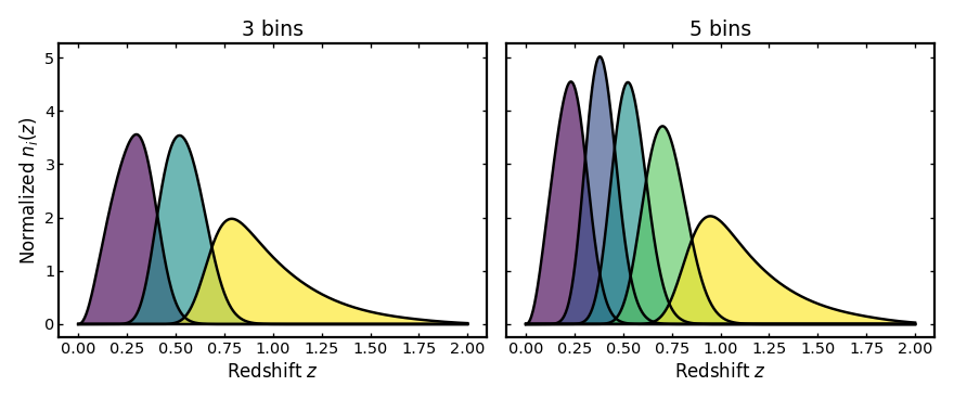
Photo-z uncertainties#
Photometric redshifts are affected by several sources of uncertainty, including statistical scatter, systematic offsets, and catastrophic outliers. These effects change how galaxies are distributed across tomographic bins and therefore modify the shapes and overlaps of the resulting distributions. The following sections illustrate how each uncertainty term affects the tomographic bins.
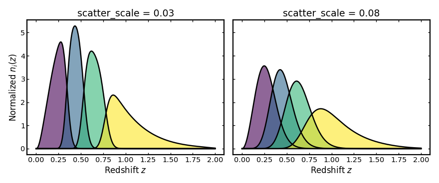
Scatter scale#
This parameter sets the width of the main photometric redshift scatter
around the mean observed redshift expected at each true redshift.
A larger scatter_scale spreads galaxies more broadly in observed
redshift, so neighboring tomographic bins overlap more strongly and the bin
edges look less sharp.
import cmasher as cmr
import matplotlib.pyplot as plt
import numpy as np

from binny import NZTomography

def plot_bins(ax, z, bin_dict, title, cmap="viridis", cmap_range=(0.0, 1.0)):
    keys = sorted(bin_dict.keys())
    colors = cmr.take_cmap_colors(
        cmap,
        len(keys),
        cmap_range=cmap_range,
        return_fmt="hex",
    )

    for i, (color, key) in enumerate(zip(colors, keys, strict=True)):
        curve = np.asarray(bin_dict[key], dtype=float)
        ax.fill_between(z, 0.0, curve, color=color, alpha=0.6, linewidth=0.0, zorder=10 + i)
        ax.plot(z, curve, color="k", linewidth=2.2, zorder=20 + i)

    ax.plot(z, np.zeros_like(z), color="k", linewidth=2.2, zorder=1000)
    ax.set_title(title)
    ax.set_xlabel("Redshift $z$")

tomo = NZTomography()
z = np.linspace(0.0, 2.0, 500)

nz = NZTomography.nz_model(
    "smail",
    z,
    z0=0.2,
    alpha=2.0,
    beta=1.0,
    normalize=True,
)

low_scatter_spec = {
    "kind": "photoz",
    "bins": {"scheme": "equipopulated", "n_bins": 4},
    "uncertainties": {"scatter_scale": 0.03},
    "normalize_bins": True,
}

high_scatter_spec = {
    "kind": "photoz",
    "bins": {"scheme": "equipopulated", "n_bins": 4},
    "uncertainties": {"scatter_scale": 0.08},
    "normalize_bins": True,
}

low_scatter_result = tomo.build_bins(z=z, nz=nz, tomo_spec=low_scatter_spec)
high_scatter_result = tomo.build_bins(z=z, nz=nz, tomo_spec=high_scatter_spec)

fig, axes = plt.subplots(1, 2, figsize=(11.0, 4.6), sharey=True)

plot_bins(axes[0], z, low_scatter_result.bins, "scatter_scale = 0.03")
axes[0].set_ylabel(r"Normalized $n_i(z)$")

plot_bins(axes[1], z, high_scatter_result.bins, "scatter_scale = 0.08")

plt.tight_layout()
(Source code, png, hires.png, pdf)

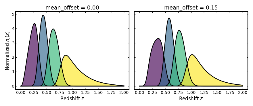
Mean offset#
This parameter adds a systematic shift to the mean observed photo-z at
fixed true redshift. A positive mean_offset moves galaxies toward higher
observed redshift than their true redshift, while a negative value would
move them lower.
import cmasher as cmr
import matplotlib.pyplot as plt
import numpy as np

from binny import NZTomography

def plot_bins(ax, z, bin_dict, title, cmap="viridis", cmap_range=(0.0, 1.0)):
    keys = sorted(bin_dict.keys())
    colors = cmr.take_cmap_colors(
        cmap,
        len(keys),
        cmap_range=cmap_range,
        return_fmt="hex",
    )

    for i, (color, key) in enumerate(zip(colors, keys, strict=True)):
        curve = np.asarray(bin_dict[key], dtype=float)
        ax.fill_between(z, 0.0, curve, color=color, alpha=0.65, linewidth=0.0, zorder=10 + i)
        ax.plot(z, curve, color="k", linewidth=2.2, zorder=20 + i)

    ax.plot(z, np.zeros_like(z), color="k", linewidth=2.2, zorder=1000)
    ax.set_title(title)
    ax.set_xlabel("Redshift $z$")

tomo = NZTomography()
z = np.linspace(0.0, 2.0, 500)

nz = NZTomography.nz_model(
    "smail",
    z,
    z0=0.2,
    alpha=2.0,
    beta=1.0,
    normalize=True,
)

zero_offset_spec = {
    "kind": "photoz",
    "bins": {"scheme": "equipopulated", "n_bins": 4},
    "uncertainties": {
        "scatter_scale": 0.04,
        "mean_offset": 0.00,
    },
    "normalize_bins": True,
}

shifted_offset_spec = {
    "kind": "photoz",
    "bins": {"scheme": "equipopulated", "n_bins": 4},
    "uncertainties": {
        "scatter_scale": 0.04,
        "mean_offset": 0.15,
    },
    "normalize_bins": True,
}

zero_offset_result = tomo.build_bins(z=z, nz=nz, tomo_spec=zero_offset_spec)
shifted_offset_result = tomo.build_bins(z=z, nz=nz, tomo_spec=shifted_offset_spec)

fig, axes = plt.subplots(1, 2, figsize=(11.0, 4.6), sharey=True)

plot_bins(axes[0], z, zero_offset_result.bins, "mean_offset = 0.00")
axes[0].set_ylabel(r"Normalized $n_i(z)$")

plot_bins(axes[1], z, shifted_offset_result.bins, "mean_offset = 0.15")

plt.tight_layout()
(Source code, png, hires.png, pdf)

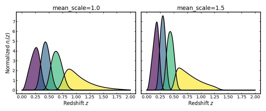
Mean scale#
This parameter rescales how the mean observed photo-z changes with true
redshift. Values above 1 make the mean observed photo-z increase more rapidly
with true redshift, while values below 1 make that increase weaker.
import cmasher as cmr
import matplotlib.pyplot as plt
import numpy as np

from binny import NZTomography

def plot_bins(ax, z, bin_dict, title, cmap="viridis", cmap_range=(0.0, 1.0)):
    keys = sorted(bin_dict.keys())
    colors = cmr.take_cmap_colors(
        cmap,
        len(keys),
        cmap_range=cmap_range,
        return_fmt="hex",
    )

    for i, (color, key) in enumerate(zip(colors, keys, strict=True)):
        curve = np.asarray(bin_dict[key], dtype=float)
        ax.fill_between(z, 0.0, curve, color=color, alpha=0.65, linewidth=0.0, zorder=10 + i)
        ax.plot(z, curve, color="k", linewidth=2.2, zorder=20 + i)

    ax.plot(z, np.zeros_like(z), color="k", linewidth=2.2, zorder=1000)
    ax.set_title(title)
    ax.set_xlabel("Redshift $z$")

tomo = NZTomography()
z = np.linspace(0.0, 2.0, 500)

nz = NZTomography.nz_model(
    "smail",
    z,
    z0=0.2,
    alpha=2.0,
    beta=1.0,
    normalize=True,
)

unit_scale_spec = {
    "kind": "photoz",
    "bins": {"scheme": "equipopulated", "n_bins": 4},
    "uncertainties": {
        "scatter_scale": 0.04,
        "mean_scale": 1.00,
    },
    "normalize_bins": True,
}

stretched_scale_spec = {
    "kind": "photoz",
    "bins": {"scheme": "equipopulated", "n_bins": 4},
    "uncertainties": {
        "scatter_scale": 0.04,
        "mean_scale": 1.50,
    },
    "normalize_bins": True,
}

unit_scale_result = tomo.build_bins(z=z, nz=nz, tomo_spec=unit_scale_spec)
stretched_scale_result = tomo.build_bins(z=z, nz=nz, tomo_spec=stretched_scale_spec)

fig, axes = plt.subplots(1, 2, figsize=(11.0, 4.6), sharey=True)

plot_bins(axes[0], z, unit_scale_result.bins, "mean_scale=1.0")
axes[0].set_ylabel(r"Normalized $n_i(z)$")

plot_bins(axes[1], z, stretched_scale_result.bins, "mean_scale=1.5")

plt.tight_layout()
(Source code, png, hires.png, pdf)

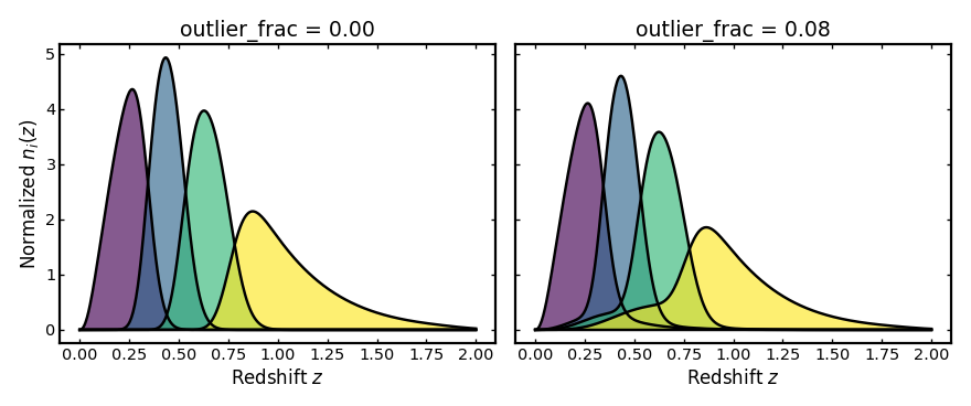
Outlier fraction#
This parameter gives the fraction of galaxies placed in the outlier
component rather than the main photo-z component.
Increasing outlier_frac puts more weight into misassigned galaxies,
which creates broader tails and stronger leakage between bins.
import cmasher as cmr
import matplotlib.pyplot as plt
import numpy as np

from binny import NZTomography

def plot_bins(ax, z, bin_dict, title, cmap="viridis", cmap_range=(0.0, 1.0)):
    keys = sorted(bin_dict.keys())
    colors = cmr.take_cmap_colors(
        cmap,
        len(keys),
        cmap_range=cmap_range,
        return_fmt="hex",
    )

    for i, (color, key) in enumerate(zip(colors, keys, strict=True)):
        curve = np.asarray(bin_dict[key], dtype=float)
        ax.fill_between(z, 0.0, curve, color=color, alpha=0.65, linewidth=0.0, zorder=10 + i)
        ax.plot(z, curve, color="k", linewidth=2.2, zorder=20 + i)

    ax.plot(z, np.zeros_like(z), color="k", linewidth=2.2, zorder=1000)
    ax.set_title(title)
    ax.set_xlabel("Redshift $z$")

tomo = NZTomography()
z = np.linspace(0.0, 2.0, 500)

nz = NZTomography.nz_model(
    "smail",
    z,
    z0=0.2,
    alpha=2.0,
    beta=1.0,
    normalize=True,
)

no_outliers_spec = {
    "kind": "photoz",
    "bins": {"scheme": "equipopulated", "n_bins": 4},
    "uncertainties": {
        "scatter_scale": 0.04,
    },
    "normalize_bins": True,
}

with_outliers_spec = {
    "kind": "photoz",
    "bins": {"scheme": "equipopulated", "n_bins": 4},
    "uncertainties": {
        "scatter_scale": 0.04,
        "outlier_frac": 0.2,
        "outlier_scatter_scale": 0.25,
        "outlier_mean_offset": 0.06,
        "outlier_mean_scale": 1.50,
    },
    "normalize_bins": True,
}

no_outliers_result = tomo.build_bins(z=z, nz=nz, tomo_spec=no_outliers_spec)
with_outliers_result = tomo.build_bins(z=z, nz=nz, tomo_spec=with_outliers_spec)

fig, axes = plt.subplots(1, 2, figsize=(11.0, 4.6), sharey=True)

plot_bins(axes[0], z, no_outliers_result.bins, "outlier_frac = 0.00")
axes[0].set_ylabel(r"Normalized $n_i(z)$")

plot_bins(axes[1], z, with_outliers_result.bins, "outlier_frac = 0.08")

plt.tight_layout()
(Source code, png, hires.png, pdf)

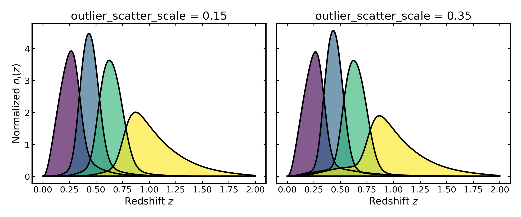
Outlier scatter scale#
This parameter sets the width of the outlier redshift distribution. A larger
outlier_scatter_scale makes the outlier population more broadly distributed
in observed redshift, so its contribution is spread over a wider range and
contaminates more bins.
import cmasher as cmr
import matplotlib.pyplot as plt
import numpy as np

from binny import NZTomography

def plot_bins(ax, z, bin_dict, title, cmap="viridis", cmap_range=(0.0, 1.0)):
    keys = sorted(bin_dict.keys())
    colors = cmr.take_cmap_colors(
        cmap,
        len(keys),
        cmap_range=cmap_range,
        return_fmt="hex",
    )

    for i, (color, key) in enumerate(zip(colors, keys, strict=True)):
        curve = np.asarray(bin_dict[key], dtype=float)
        ax.fill_between(z, 0.0, curve, color=color, alpha=0.65, linewidth=0.0, zorder=10 + i)
        ax.plot(z, curve, color="k", linewidth=2.2, zorder=20 + i)

    ax.plot(z, np.zeros_like(z), color="k", linewidth=2.2, zorder=1000)
    ax.set_title(title)
    ax.set_xlabel("Redshift $z$")

tomo = NZTomography()
z = np.linspace(0.0, 2.0, 500)

nz = NZTomography.nz_model(
    "smail",
    z,
    z0=0.2,
    alpha=2.0,
    beta=1.0,
    normalize=True,
)

narrow_outlier_spec = {
    "kind": "photoz",
    "bins": {"scheme": "equipopulated", "n_bins": 4},
    "uncertainties": {
        "scatter_scale": 0.04,
        "outlier_frac": 0.2,
        "outlier_scatter_scale": 0.15,
        "outlier_mean_offset": 0.06,
        "outlier_mean_scale": 1.00,
    },
    "normalize_bins": True,
}

broad_outlier_spec = {
    "kind": "photoz",
    "bins": {"scheme": "equipopulated", "n_bins": 4},
    "uncertainties": {
        "scatter_scale": 0.04,
        "outlier_frac": 0.2,
        "outlier_scatter_scale": 0.35,
        "outlier_mean_offset": 0.06,
        "outlier_mean_scale": 1.00,
    },
    "normalize_bins": True,
}

narrow_outlier_result = tomo.build_bins(z=z, nz=nz, tomo_spec=narrow_outlier_spec)
broad_outlier_result = tomo.build_bins(z=z, nz=nz, tomo_spec=broad_outlier_spec)

fig, axes = plt.subplots(1, 2, figsize=(11.0, 4.6), sharey=True)

plot_bins(axes[0], z, narrow_outlier_result.bins, "outlier_scatter_scale = 0.15")
axes[0].set_ylabel(r"Normalized $n_i(z)$")

plot_bins(axes[1], z, broad_outlier_result.bins, "outlier_scatter_scale = 0.35")

plt.tight_layout()
(Source code, png, hires.png, pdf)

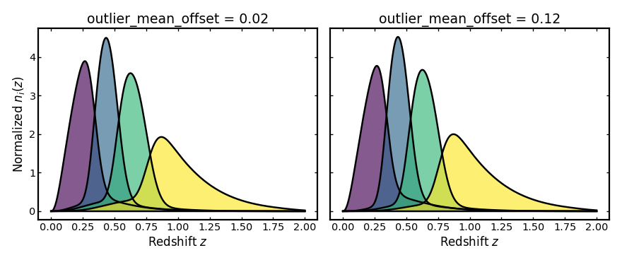
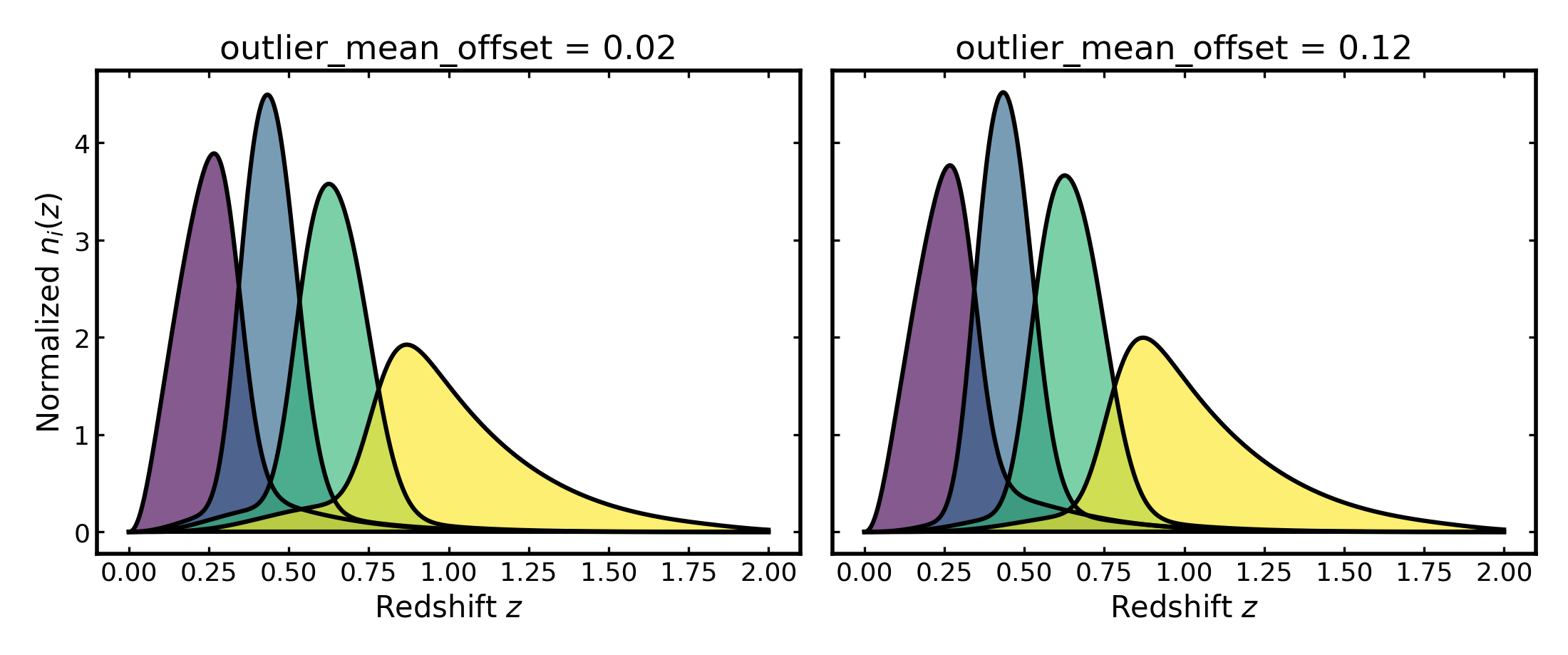
Outlier mean offset#
This parameter shifts the mean observed redshift of the outlier
population relative to the main photo-z population.
Increasing outlier_mean_offset moves the outlier population farther
from the redshift range occupied by the main population.
import cmasher as cmr
import matplotlib.pyplot as plt
import numpy as np

from binny import NZTomography

def plot_bins(ax, z, bin_dict, title, cmap="viridis", cmap_range=(0.0, 1.0)):
    keys = sorted(bin_dict.keys())
    colors = cmr.take_cmap_colors(
        cmap,
        len(keys),
        cmap_range=cmap_range,
        return_fmt="hex",
    )

    for i, (color, key) in enumerate(zip(colors, keys, strict=True)):
        curve = np.asarray(bin_dict[key], dtype=float)
        ax.fill_between(z, 0.0, curve, color=color, alpha=0.65, linewidth=0.0, zorder=10 + i)
        ax.plot(z, curve, color="k", linewidth=2.2, zorder=20 + i)

    ax.plot(z, np.zeros_like(z), color="k", linewidth=2.2, zorder=1000)
    ax.set_title(title)
    ax.set_xlabel("Redshift $z$")

tomo = NZTomography()
z = np.linspace(0.0, 2.0, 500)

nz = NZTomography.nz_model(
    "smail",
    z,
    z0=0.2,
    alpha=2.0,
    beta=1.0,
    normalize=True,
)

small_outlier_shift_spec = {
    "kind": "photoz",
    "bins": {"scheme": "equipopulated", "n_bins": 4},
    "uncertainties": {
        "scatter_scale": 0.04,
        "outlier_frac": 0.2,
        "outlier_scatter_scale": 0.25,
        "outlier_mean_offset": 0.02,
        "outlier_mean_scale": 1.00,
    },
    "normalize_bins": True,
}

large_outlier_shift_spec = {
    "kind": "photoz",
    "bins": {"scheme": "equipopulated", "n_bins": 4},
    "uncertainties": {
        "scatter_scale": 0.04,
        "outlier_frac": 0.2,
        "outlier_scatter_scale": 0.25,
        "outlier_mean_offset": 0.2,
        "outlier_mean_scale": 1.00,
    },
    "normalize_bins": True,
}

small_outlier_shift_result = tomo.build_bins(z=z, nz=nz, tomo_spec=small_outlier_shift_spec)
large_outlier_shift_result = tomo.build_bins(z=z, nz=nz, tomo_spec=large_outlier_shift_spec)

fig, axes = plt.subplots(1, 2, figsize=(11.0, 4.6), sharey=True)

plot_bins(axes[0], z, small_outlier_shift_result.bins, "outlier_mean_offset = 0.02")
axes[0].set_ylabel(r"Normalized $n_i(z)$")

plot_bins(axes[1], z, large_outlier_shift_result.bins, "outlier_mean_offset = 0.12")

plt.tight_layout()
(Source code, png, hires.png, pdf)

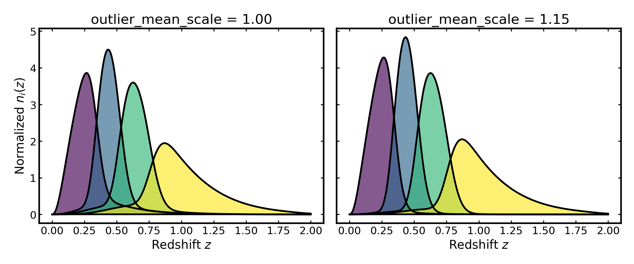
Outlier mean scale#
This parameter rescales how the mean observed redshift of the outlier
population changes with true redshift. A value of 1 gives the default
scaling, while values above or below 1 make the outlier mean increase
more quickly or more slowly with redshift.
import cmasher as cmr
import matplotlib.pyplot as plt
import numpy as np

from binny import NZTomography

def plot_bins(ax, z, bin_dict, title, cmap="viridis", cmap_range=(0.0, 1.0)):
    keys = sorted(bin_dict.keys())
    colors = cmr.take_cmap_colors(
        cmap,
        len(keys),
        cmap_range=cmap_range,
        return_fmt="hex",
    )

    for i, (color, key) in enumerate(zip(colors, keys, strict=True)):
        curve = np.asarray(bin_dict[key], dtype=float)
        ax.fill_between(z, 0.0, curve, color=color, alpha=0.65, linewidth=0.0, zorder=10 + i)
        ax.plot(z, curve, color="k", linewidth=2.2, zorder=20 + i)

    ax.plot(z, np.zeros_like(z), color="k", linewidth=2.2, zorder=1000)
    ax.set_title(title)
    ax.set_xlabel("Redshift $z$")

tomo = NZTomography()
z = np.linspace(0.0, 2.0, 500)

nz = NZTomography.nz_model(
    "smail",
    z,
    z0=0.2,
    alpha=2.0,
    beta=1.0,
    normalize=True,
)

unit_outlier_scale_spec = {
    "kind": "photoz",
    "bins": {"scheme": "equipopulated", "n_bins": 4},
    "uncertainties": {
        "scatter_scale": 0.04,
        "outlier_frac": 0.2,
        "outlier_scatter_scale": 0.25,
        "outlier_mean_offset": 0.06,
        "outlier_mean_scale": 1.00,
    },
    "normalize_bins": True,
}

stretched_outlier_scale_spec = {
    "kind": "photoz",
    "bins": {"scheme": "equipopulated", "n_bins": 4},
    "uncertainties": {
        "scatter_scale": 0.04,
        "outlier_frac": 0.06,
        "outlier_scatter_scale": 0.25,
        "outlier_mean_offset": 0.06,
        "outlier_mean_scale": 1.5,
    },
    "normalize_bins": True,
}

unit_outlier_scale_result = tomo.build_bins(z=z, nz=nz, tomo_spec=unit_outlier_scale_spec)
stretched_outlier_scale_result = tomo.build_bins(z=z, nz=nz, tomo_spec=stretched_outlier_scale_spec)

fig, axes = plt.subplots(1, 2, figsize=(11.0, 4.6), sharey=True)

plot_bins(axes[0], z, unit_outlier_scale_result.bins, "outlier_mean_scale = 1.00")
axes[0].set_ylabel(r"Normalized $n_i(z)$")

plot_bins(axes[1], z, stretched_outlier_scale_result.bins, "outlier_mean_scale = 1.15")

plt.tight_layout()
(Source code, png, hires.png, pdf)

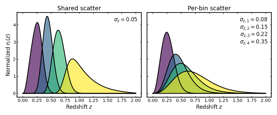
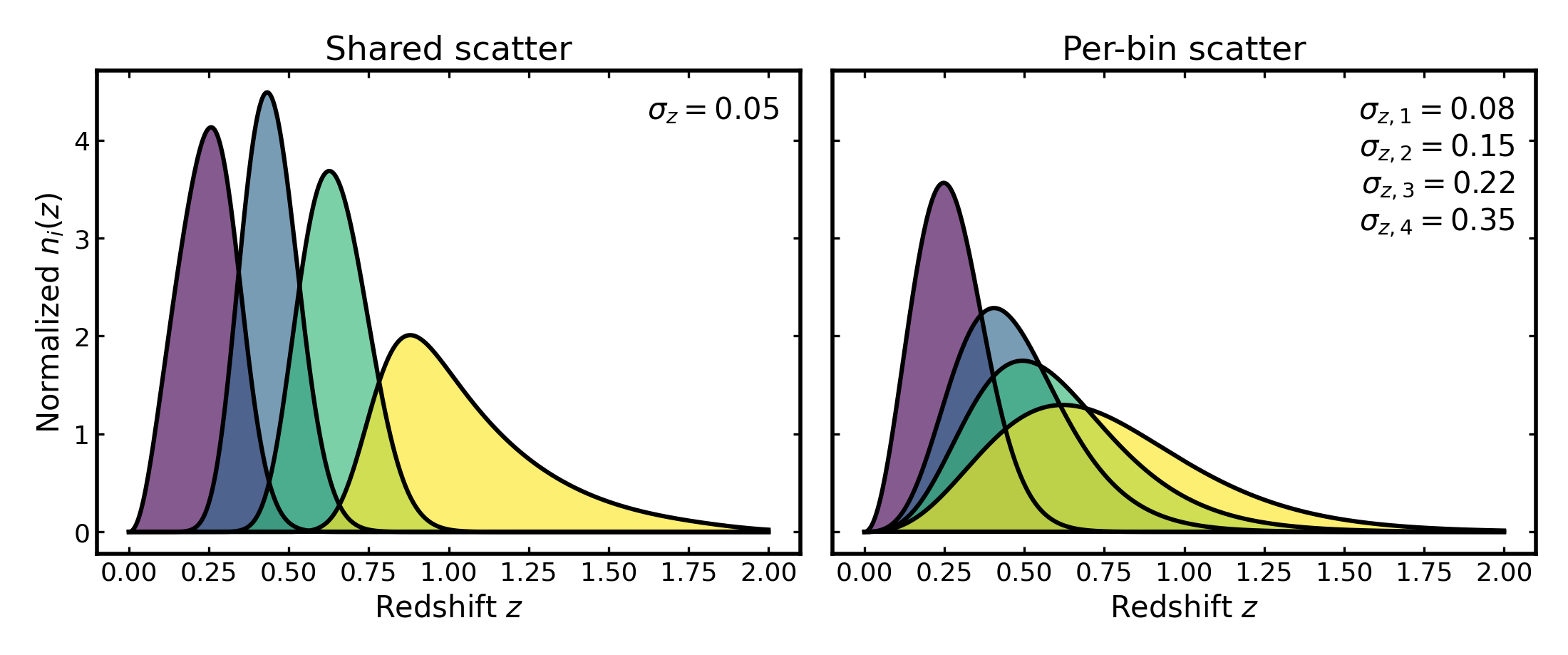
Per-bin versus shared uncertainties#
Photo-z uncertainty parameters can be given either as a single value applied to all tomographic bins or as a list with one value per bin. This is useful because some analyses assume a shared uncertainty model across the full sample, while others allow the uncertainty parameters to vary from bin to bin.
The example below compares these two cases using the same binning setup. On
the left, all bins use the same scatter_scale. On the right, each bin is
assigned its own scatter level.
import cmasher as cmr
import matplotlib.pyplot as plt
import numpy as np

from binny import NZTomography

def plot_bins(
    ax,
    z,
    bin_dict,
    title,
    scatter_text,
    cmap="viridis",
    cmap_range=(0.0, 1.0),
):
    keys = sorted(bin_dict.keys())
    colors = cmr.take_cmap_colors(
        cmap,
        len(keys),
        cmap_range=cmap_range,
        return_fmt="hex",
    )

    for i, (color, key) in enumerate(zip(colors, keys, strict=True)):
        curve = np.asarray(bin_dict[key], dtype=float)
        ax.fill_between(
            z,
            0.0,
            curve,
            color=color,
            alpha=0.65,
            linewidth=0.0,
            zorder=10 + i,
        )
        ax.plot(
            z,
            curve,
            color="k",
            linewidth=2.2,
            zorder=20 + i,
        )

    ax.plot(z, np.zeros_like(z), color="k", linewidth=2.2, zorder=1000)
    ax.set_title(title)
    ax.set_xlabel("Redshift $z$")

    ax.text(
        0.97,
        0.95,
        scatter_text,
        transform=ax.transAxes,
        ha="right",
        va="top",
        bbox=dict(
            boxstyle="round",
            facecolor="white",
            alpha=0.9,
            edgecolor="none",
        ),
    )

tomo = NZTomography()
z = np.linspace(0.0, 2.0, 500)

nz = NZTomography.nz_model(
    "smail",
    z,
    z0=0.2,
    alpha=2.0,
    beta=1.0,
    normalize=True,
)

shared_uncertainty_spec = {
    "kind": "photoz",
    "bins": {"scheme": "equipopulated", "n_bins": 4},
    "uncertainties": {
        "scatter_scale": 0.05,
    },
    "normalize_bins": True,
}

per_bin_scatter = [0.08, 0.15, 0.22, 0.35]

per_bin_uncertainty_spec = {
    "kind": "photoz",
    "bins": {"scheme": "equipopulated", "n_bins": 4},
    "uncertainties": {
        "scatter_scale": per_bin_scatter,
    },
    "normalize_bins": True,
}

shared_result = tomo.build_bins(z=z, nz=nz, tomo_spec=shared_uncertainty_spec)
per_bin_result = tomo.build_bins(z=z, nz=nz, tomo_spec=per_bin_uncertainty_spec)

shared_text = r"$\sigma_z = {:.2f}$".format(
    shared_uncertainty_spec["uncertainties"]["scatter_scale"]
)

per_bin_text = "\n".join(
    rf"$\sigma_{{z,{i+1}}} = {val:.2f}$"
    for i, val in enumerate(per_bin_scatter)
)

fig, axes = plt.subplots(1, 2, figsize=(11.0, 4.6), sharey=True)

plot_bins(
    axes[0],
    z,
    shared_result.bins,
    "Shared scatter",
    shared_text,
)
axes[0].set_ylabel(r"Normalized $n_i(z)$")

plot_bins(
    axes[1],
    z,
    per_bin_result.bins,
    "Per-bin scatter",
    per_bin_text,
)

plt.tight_layout()
(Source code, png, hires.png, pdf)

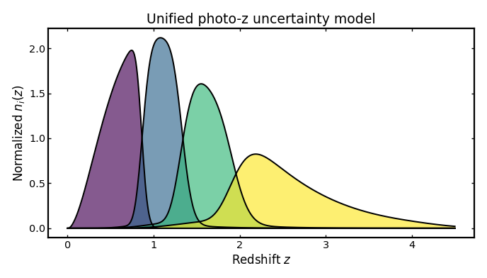
Unified uncertainty model#
This combines all photo-z uncertainty terms at once: the width of the main scatter, a systematic shift in the mean redshift relation, a rescaling of that relation, and a separate outlier population with its own fraction, offset, scaling, and scatter. In practice this is the most realistic setup, because real photometric redshift errors usually include both a main population of roughly correct estimates and a smaller population of catastrophic outliers.
The example below follows the full schema style and uses per-bin values for all uncertainty ingredients.
import cmasher as cmr
import matplotlib.pyplot as plt
import numpy as np

from binny import NZTomography

def plot_bins(ax, z, bin_dict, title, cmap="viridis", cmap_range=(0.0, 1.0)):
    keys = sorted(bin_dict.keys())
    colors = cmr.take_cmap_colors(
        cmap,
        len(keys),
        cmap_range=cmap_range,
        return_fmt="hex",
    )

    for i, (color, key) in enumerate(zip(colors, keys, strict=True)):
        curve = np.asarray(bin_dict[key], dtype=float)
        ax.fill_between(
            z,
            0.0,
            curve,
            color=color,
            alpha=0.65,
            linewidth=0.0,
            zorder=10 + i,
        )
        ax.plot(
            z,
            curve,
            color="k",
            linewidth=1.8,
            zorder=20 + i,
        )

    ax.plot(z, np.zeros_like(z), color="k", linewidth=1.8, zorder=1000)
    ax.set_title(title)
    ax.set_xlabel("Redshift $z$")
    ax.set_ylabel(r"Normalized $n_i(z)$")

tomo = NZTomography()

z = np.linspace(0.0, 4.5, 500)

nz = NZTomography.nz_model(
    "smail",
    z,
    z0=0.5,
    alpha=2.0,
    beta=1.0,
    normalize=True,
)

unified_uncertainty_spec = {
    "kind": "photoz",
    "bins": {
        "scheme": "equipopulated",
        "n_bins": 4,
    },
    "uncertainties": {
        "scatter_scale": [0.03, 0.04, 0.05, 0.06],
        "mean_offset": [0.00, 0.01, 0.01, 0.02],
        "mean_scale": [1.00, 1.00, 1.00, 1.00],
        "outlier_frac": [0.00, 0.05, 0.1, 0.15],
        "outlier_scatter_scale": [0.00, 0.20, 0.25, 0.30],
        "outlier_mean_offset": [0.00, 0.05, 0.05, 0.08],
        "outlier_mean_scale": [1.00, 1.00, 1.00, 1.00],
    },
    "normalize_bins": True,
}

unified_result = tomo.build_bins(
    z=z,
    nz=nz,
    tomo_spec=unified_uncertainty_spec,
)

fig, ax = plt.subplots(figsize=(8.6, 4.9))
plot_bins(
    ax,
    z,
    unified_result.bins,
    title="Unified photo-z uncertainty model",
)
plt.tight_layout()
(Source code, png, hires.png, pdf)
Inspecting the returned bins#
The bin construction routine returns a structured result object that contains the parent redshift distribution, the individual tomographic bins, and the resolved configuration used to build them. The example below demonstrates how to access and inspect these components programmatically.
import numpy as np
from binny import NZTomography

tomo = NZTomography()

z = np.linspace(0.0, 2.0, 500)

nz = NZTomography.nz_model(
    "smail",
    z,
    z0=0.5,
    alpha=2.0,
    beta=1.0,
    normalize=True,
)

spec = {
    "kind": "photoz",
    "bins": {
        "scheme": "equipopulated",
        "n_bins": 4,
    },
    "uncertainties": {
        "scatter_scale": [0.03, 0.04, 0.05, 0.06],
        "mean_offset": [0.00, 0.01, 0.01, 0.02],
        "mean_scale": [1.00, 1.00, 1.00, 1.00],
        "outlier_frac": [0.00, 0.02, 0.03, 0.05],
        "outlier_scatter_scale": [0.00, 0.20, 0.25, 0.30],
        "outlier_mean_offset": [0.00, 0.05, 0.05, 0.08],
        "outlier_mean_scale": [1.00, 1.00, 1.00, 1.00],
    },
    "normalize_bins": True,
}

result = tomo.build_bins(z=z, nz=nz, tomo_spec=spec)

print("bin keys:", list(result.bins.keys()))
print("parent shape:", result.nz.shape)
print("bin 0 shape:", result.bins[0].shape)
print("resolved scheme:", result.spec["bins"]["scheme"])
Notes#
These examples use
binny.NZTomography.build_bins()with a compacttomo_specmapping.Photometric tomography requires an
uncertaintiesblock in addition to the parentnzmodel and binning setup.The uncertainty examples above vary one ingredient at a time so that the role of each parameter can be seen more clearly.
The unified example follows the full schema and includes per-bin values for both the main and outlier components.
The plotting style here uses filled tomographic curves with black outlines, matching the broader Binny visual style more closely than plain line plots.