 Parent n(z) models#
This page provides simple, executable examples showing how to use
binny.NZTomography to inspect and evaluate theoretical parent
redshift distributions \(n(z)\) available through the Binny registry.
These examples focus on parent distributions, not tomographic bins. They are useful for exploring the shape of built-in models before using them in a tomography workflow.
All plotting examples below are executable via .. plot::.
Listing available n(z) models#
Before evaluating a specific model, it can be helpful to inspect which
parent redshift distributions are currently registered in Binny. This
gives a quick overview of the built-in options available through
binny.NZTomography.list_nz_models().
from binny import NZTomography

models = NZTomography.list_nz_models()

print(f"Found {len(models)} registered n(z) models:")
for name in models:
    print(f" - {name}")
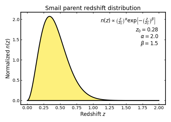
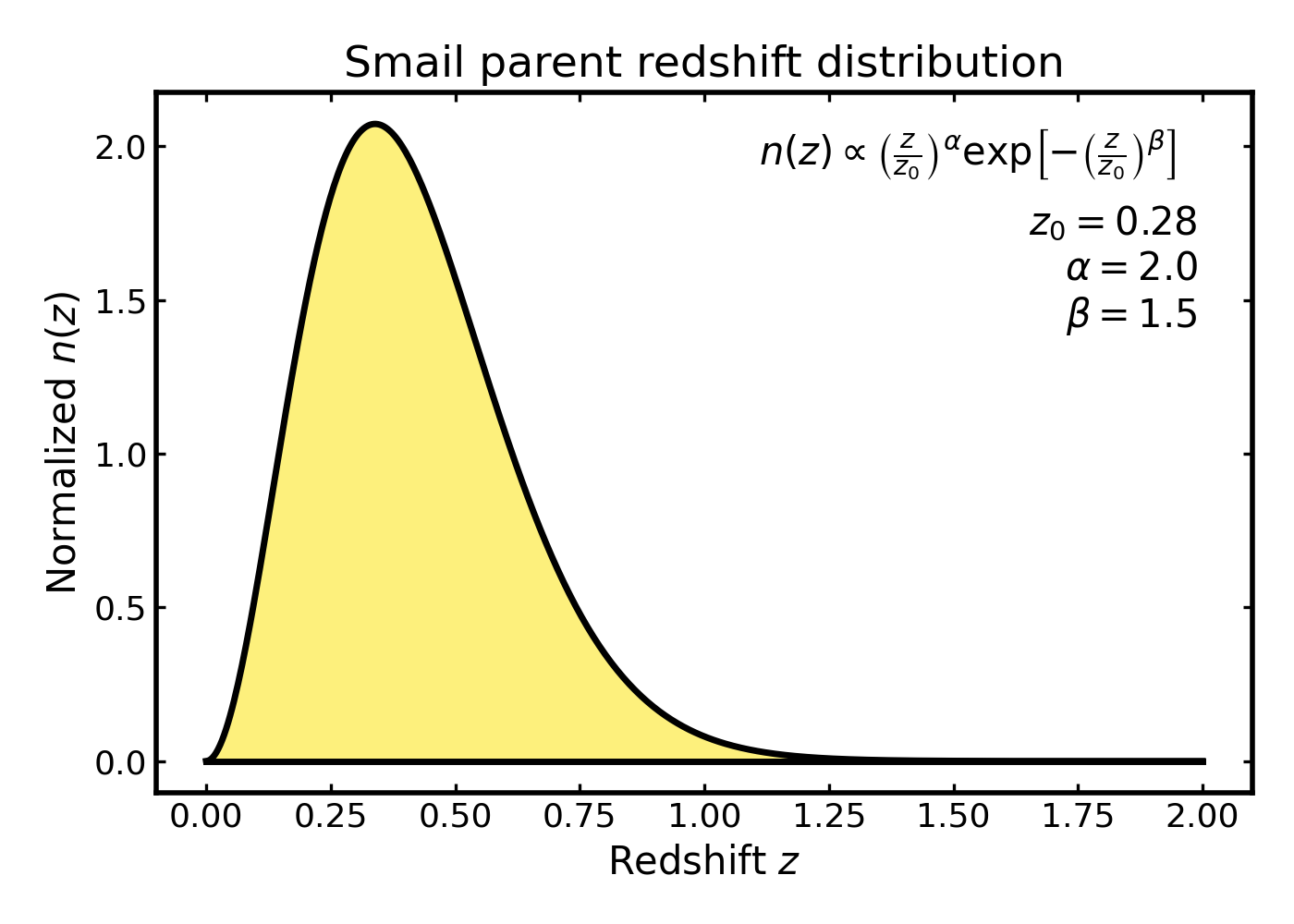
Basic Smail model#
We begin with a standard Smail distribution, which is a common choice for survey-like galaxy redshift distributions. It provides a smooth, single-peaked shape and is often used as a simple baseline model in forecasting studies.
import cmasher as cmr
import matplotlib.pyplot as plt
import numpy as np

from binny import NZTomography

z = np.linspace(0.0, 2.0, 500)

z0 = 0.28
alpha = 2.0
beta = 1.5

nz_smail = NZTomography.nz_model(
    "smail",
    z,
    z0=z0,
    alpha=alpha,
    beta=beta,
    normalize=True,
)

color_smail = cmr.take_cmap_colors(
    "viridis",
    3,
    cmap_range=(0.0, 1.0),
    return_fmt="hex",
)[-1]

fig, ax = plt.subplots(figsize=(7, 5))

ax.fill_between(
    z,
    0.0,
    nz_smail,
    color=color_smail,
    alpha=0.6,
    linewidth=0.0,
    zorder=10,
)
ax.plot(z, nz_smail, color="k", linewidth=2.5, zorder=20)
ax.plot(z, np.zeros_like(z), color="k", linewidth=2.5, zorder=100)

formula_text = (
    r"$n(z)\propto\left(\frac{z}{z_0}\right)^{\alpha}"
    r"\exp\!\left[-\left(\frac{z}{z_0}\right)^{\beta}\right]$"
)

param_text = (
    r"$z_0 = {:.2f}$" "\n"
    r"$\alpha = {:.1f}$" "\n"
    r"$\beta = {:.1f}$"
).format(z0, alpha, beta)

ax.text(
    0.55,
    0.95,
    formula_text,
    transform=ax.transAxes,
    ha="left",
    va="top",
)

ax.text(
    0.95,
    0.84,
    param_text,
    transform=ax.transAxes,
    ha="right",
    va="top",
)

ax.set_xlabel("Redshift $z$")
ax.set_ylabel(r"Normalized $n(z)$")
ax.set_title("Smail parent redshift distribution")

plt.tight_layout()
(Source code, png, hires.png, pdf)

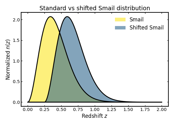
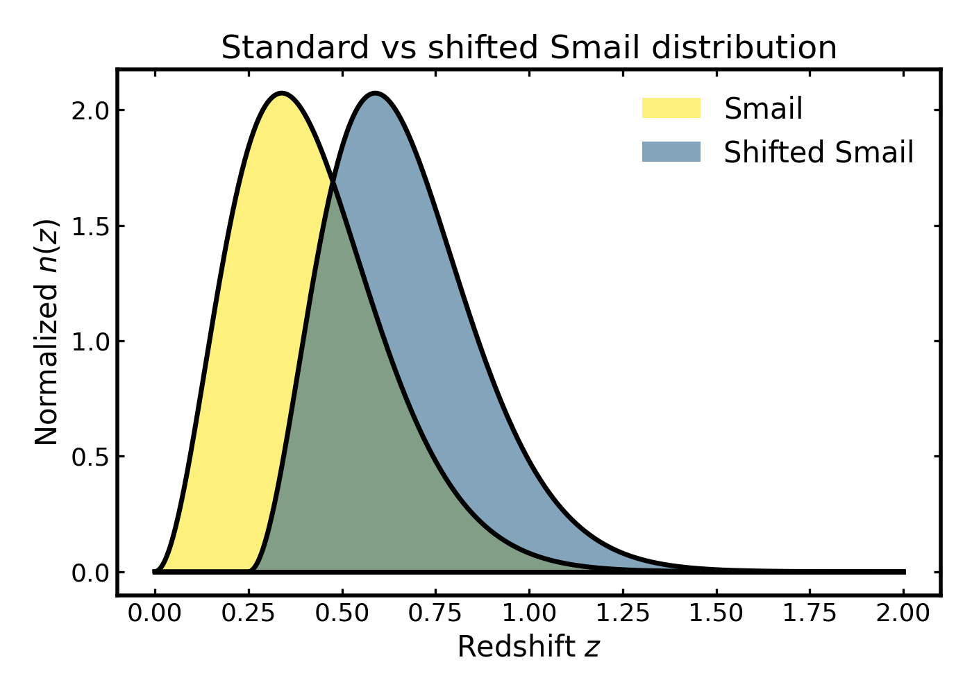
Shifted Smail model#
The shifted Smail model is a small variation of the standard Smail distribution in which the entire profile is moved toward higher redshift by a fixed offset. This can be useful when modeling samples that have a delayed onset in redshift, for example when low-redshift galaxies are removed by a selection cut or when the survey sensitivity effectively shifts the observable population to higher redshift.
In the example below we compare the standard Smail model with a shifted version to illustrate how the overall shape remains similar while the peak and support move to larger redshift.
import cmasher as cmr
import matplotlib.pyplot as plt
import numpy as np

from binny import NZTomography

z = np.linspace(0.0, 2.0, 500)

nz_standard = NZTomography.nz_model(
    "smail",
    z,
    z0=0.28,
    alpha=2.0,
    beta=1.5,
    normalize=True,
)

nz_shifted = NZTomography.nz_model(
    "shifted_smail",
    z,
    z0=0.28,
    alpha=2.0,
    beta=1.5,
    z_shift=0.25,
    normalize=True,
)

colors = cmr.take_cmap_colors(
    "viridis_r",
    4,
    cmap_range=(0.0, 1.0),
    return_fmt="hex",
)
color_standard, _, color_shifted, _ = colors

fig, ax = plt.subplots(figsize=(7.0, 5.0))

ax.fill_between(
    z,
    0.0,
    nz_standard,
    color=color_standard,
    alpha=0.6,
    linewidth=0.0,
    zorder=10,
    label="Smail",
)
ax.plot(z, nz_standard, color="k", linewidth=2.5, zorder=20)

ax.fill_between(
    z,
    0.0,
    nz_shifted,
    color=color_shifted,
    alpha=0.6,
    linewidth=0.0,
    zorder=11,
    label="Shifted Smail",
)
ax.plot(z, nz_shifted, color="k", linewidth=2.5, zorder=21)
ax.plot(z, np.zeros_like(z), color="k", linewidth=2.5, zorder=100)

ax.set_xlabel("Redshift $z$")
ax.set_ylabel(r"Normalized $n(z)$")
ax.set_title("Standard vs shifted Smail distribution")
ax.legend(frameon=False, loc="upper right")

plt.tight_layout()
(Source code, png, hires.png, pdf)

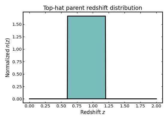
Top-hat distribution#
Not all parent distributions need to be smooth. In some cases it is useful to work with a compact-support model that is non-zero only over a fixed redshift interval. The top-hat model is therefore a convenient toy example for testing and visual comparisons.
import cmasher as cmr
import matplotlib.pyplot as plt
import numpy as np

from binny import NZTomography

z = np.linspace(0.0, 2.0, 500)

nz_tophat = NZTomography.nz_model(
    "tophat",
    z,
    zmin=0.6,
    zmax=1.2,
    normalize=True,
)

color_tophat = cmr.take_cmap_colors(
    "viridis",
    3,
    cmap_range=(0.0, 1.0),
    return_fmt="hex",
)[1]

fig, ax = plt.subplots(figsize=(7.0, 5.0))

ax.fill_between(
    z,
    0.0,
    nz_tophat,
    color=color_tophat,
    alpha=0.6,
    linewidth=0.0,
    zorder=10,
)
ax.plot(z, nz_tophat, color="k", linewidth=2.5, zorder=20)
ax.plot(z, np.zeros_like(z), color="k", linewidth=2.5, zorder=100)

ax.set_xlabel("Redshift $z$")
ax.set_ylabel(r"Normalized $n(z)$")
ax.set_title("Top-hat parent redshift distribution")

plt.tight_layout()
(Source code, png, hires.png, pdf)
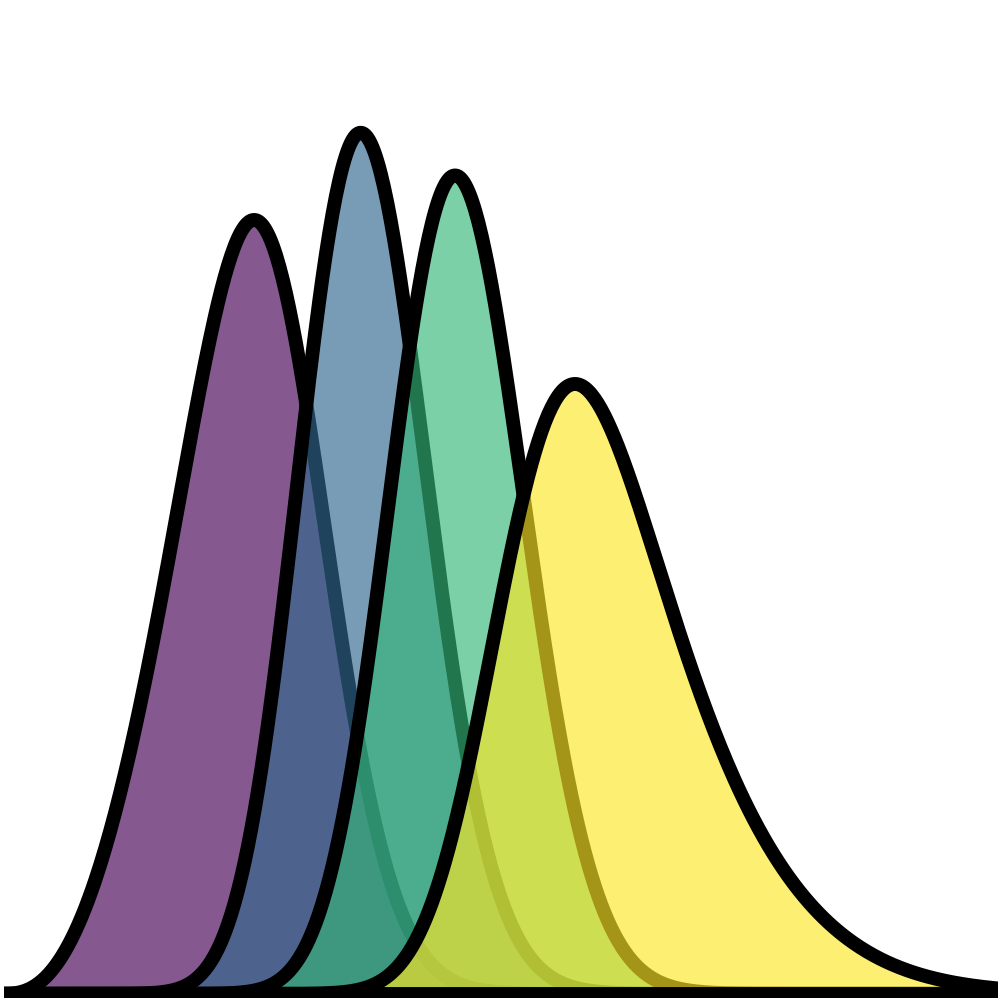
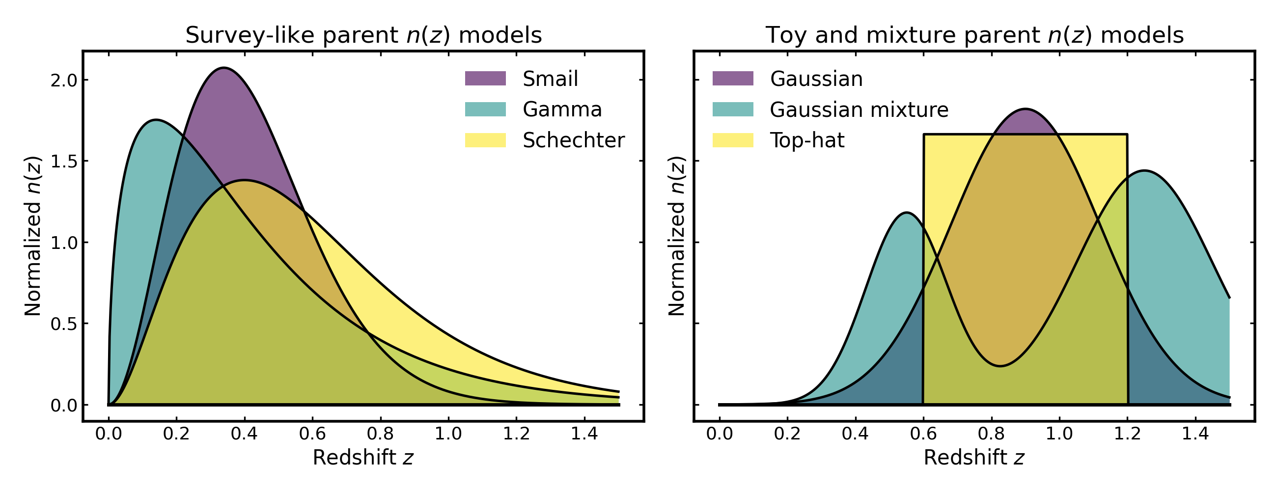
Comparing registered parent n(z) models#
Different parent \(n(z)\) models can produce noticeably different shapes, even when they are all normalized on the same redshift grid. In this example we compare six built-in models. To keep the figure readable, they are grouped into two panels: one showing survey-like shapes and one showing simpler toy or mixture-based examples.
import cmasher as cmr
import matplotlib.pyplot as plt
import numpy as np

from binny import NZTomography

def plot_parent_models(ax, z, model_curves, title):
    colors = cmr.take_cmap_colors(
        "viridis",
        3,
        cmap_range=(0.0, 1.0),
        return_fmt="hex",
    )

    for i, ((label, nz_values), color) in enumerate(
        zip(model_curves, colors, strict=True)
    ):
        ax.fill_between(
            z,
            0.0,
            nz_values,
            color=color,
            alpha=0.6,
            linewidth=0.0,
            zorder=10 + i,
            label=label,
        )
        ax.plot(
            z,
            nz_values,
            color="k",
            linewidth=1.8,
            zorder=20 + i,
        )

    ax.plot(z, np.zeros_like(z), color="k", linewidth=2.5, zorder=1000)

    ax.set_title(title)
    ax.set_xlabel("Redshift $z$")
    ax.set_ylabel(r"Normalized $n(z)$")
    ax.legend(frameon=False, loc="best")

z = np.linspace(0.0, 1.5, 500)

panel1_models = [
    (
        "Smail",
        NZTomography.nz_model(
            "smail",
            z,
            z0=0.28,
            alpha=2.0,
            beta=1.5,
            normalize=True,
        ),
    ),
    (
        "Gamma",
        NZTomography.nz_model(
            "gamma",
            z,
            k=1.5,
            theta=0.28,
            normalize=True,
        ),
    ),
    (
        "Schechter",
        NZTomography.nz_model(
            "schechter",
            z,
            z0=0.2,
            alpha=2.0,
            normalize=True,
        ),
    ),
]


panel2_models = [
    (
        "Gaussian",
        NZTomography.nz_model(
            "gaussian",
            z,
            mu=0.9,
            sigma=0.22,
            normalize=True,
        ),
    ),
    (
        "Gaussian mixture",
        NZTomography.nz_model(
            "gaussian_mixture",
            z,
            mus=np.array([0.55, 1.25]),
            sigmas=np.array([0.12, 0.20]),
            weights=np.array([0.45, 0.55]),
            normalize=True,
        ),
    ),
    (
        "Top-hat",
        NZTomography.nz_model(
            "tophat",
            z,
            zmin=0.6,
            zmax=1.2,
            normalize=True,
        ),
    ),
]


fig, axes = plt.subplots(1, 2, figsize=(13.0, 5.0), sharey=True)

plot_parent_models(axes[0], z, panel1_models, "Survey-like parent $n(z)$ models")
plot_parent_models(axes[1], z, panel2_models, "Toy and mixture parent $n(z)$ models")

plt.tight_layout()
(Source code, png, hires.png, pdf)

Inspecting model values directly#
In addition to plotting a parent distribution, you can also inspect the returned values directly. This can be useful when checking array shapes, verifying normalization behavior, or passing the evaluated model into a later part of a tomography workflow.
import numpy as np

from binny import NZTomography

z = np.linspace(0.0, 2.0, 500)

nz = NZTomography.nz_model(
    "gaussian",
    z,
    mu=1.0,
    sigma=0.25,
    normalize=True,
)

print("z grid:")
print(z)
print()
print("n(z) values:")
print(nz)
print()
print("Shape:", nz.shape)
print("All non-negative:", bool(np.all(nz >= 0.0)))
Notes#
These examples use
binny.NZTomography.nz_model(), which evaluates a registered parent redshift distribution on a supplied redshift grid.Setting
normalize=Truemakes the model integrate to unity over the provided grid.These are parent distributions, not tomographic bins. To construct tomographic bins from a parent \(n(z)\), see the tomography examples in Examples.
If you are unsure about the workflow for constructing tomographic bins, see the Workflow page for an overview of the typical steps involved.