Analytic parent n(z) models

Why model a parent \(n(z)\)?

In many forecasting or methodology studies, the starting point is not a fully observed galaxy catalog but an analytic or semi-analytic description of the source population. A parent distribution \(n(z)\) is useful because it provides a compact way to encode the overall redshift structure of the sample before introducing tomographic cuts, photo-\(z\) uncertainties, or survey-specific selection effects.

This has several advantages:

• it provides a smooth, controllable baseline population,

• it makes synthetic or survey-inspired tests reproducible,

• it allows one to vary depth or shape parameters in a simple way,

• and it separates the description of the overall galaxy population from the later step of constructing tomographic bins.

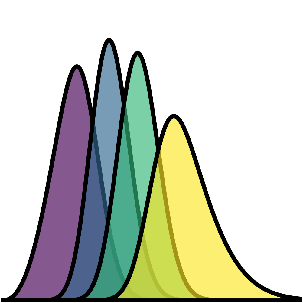
Conceptually, Binny treats the parent \(n(z)\) as the continuous distribution from which the tomographic bin curves are derived. The bin curves therefore inherit many of their qualitative properties from the choice of parent model.

What is implemented in Binny

Binny provides a registry of named parent redshift-distribution models. At present, the following models are implemented:

• smail

• shifted_smail

• gaussian

• gaussian_mixture

• gamma

• schechter

• lognormal

• skew_normal

• student_t

• tophat

• luminosity_function

These models are exposed through the parent-distribution registry and can be evaluated through binny.NZTomography.nz_model().

The purpose of the registry is not to claim that all of these models are equally realistic for survey forecasting. Rather, Binny supports a small family of parent distributions because different use cases benefit from different levels of realism, simplicity, or flexibility. Some models are well suited to survey-like baseline populations, while others are useful as controlled toy models for testing, pedagogy, or stress tests of a binning workflow.

Survey-like baseline models

Among the implemented models, the Smail distribution [Smail1994] is the most natural default for many survey-like applications. It is widely used in forecasting because it provides a smooth, unimodal distribution with a rising low-redshift part and a decaying high-redshift tail. This makes it a convenient phenomenological description of a magnitude-limited galaxy sample.

In Binny, the Smail-like parent distribution is parameterized through a redshift scale \(z_0\) and two shape parameters, usually written as \(\alpha\) and \(\beta\). In schematic form,

\[n(z) \propto \left(\frac{z}{z_0}\right)^{\alpha} \exp\!\left[-\left(\frac{z}{z_0}\right)^{\beta}\right].\]

The role of these parameters is intuitive:

• \(z_0\) sets the characteristic redshift scale,

• \(\alpha\) controls how rapidly the distribution rises at low redshift,

• \(\beta\) controls how quickly the high-redshift tail falls off.

This functional form is especially useful because it is simple enough to work with analytically and numerically, while still being flexible enough to mimic the broad shape of galaxy samples encountered in many forecasting studies.

The typical values of the shape parameters are not arbitrary. In many forecasting applications one often encounters values around

\[\alpha \approx 2, \qquad \beta \sim 1\text{–}1.5.\]

This choice reflects two broad features of magnitude-limited galaxy samples.

At low redshift, the number of galaxies in a thin redshift shell scales approximately with the comoving volume element,

\[\mathrm{d}V \propto z^2\, \mathrm{d}z,\]

which is the leading-order behavior of the cosmological volume element for small redshift. If the galaxy population evolves slowly over this range, the redshift distribution therefore rises approximately as \(n(z) \propto z^2\).

At higher redshift, the distribution must eventually decline. This turnover is primarily driven by survey selection effects. As distance increases, galaxies appear fainter and a magnitude-limited survey progressively loses objects beyond a characteristic depth set by the survey flux limit and the galaxy luminosity function. The exponential factor in the Smail model mimics this suppression, with the parameter \(\beta\) controlling how sharply the high-redshift tail falls.

Values of \(\beta\) around unity therefore produce a gradual survey-like decline, while larger values lead to a steeper cutoff.

The parameter \(z_0\) sets the characteristic redshift scale at which the distribution transitions from the low-redshift power-law rise to the high-redshift exponential suppression. The actual peak of the distribution occurs at

\[z_{\rm peak} = z_0 \left(\frac{\alpha}{\beta}\right)^{1/\beta},\]

so \(z_0\) should be interpreted as a scale parameter rather than the peak location itself.

In practice these parameters are rarely interpreted as physical constants. Instead, they serve as convenient phenomenological controls that allow the analytic distribution to reproduce the broad statistical shape of a magnitude-limited galaxy population.

For this reason, the Smail model is often a natural first choice when one wants a survey-like parent \(n(z)\) without committing to a more complicated catalog-level model.

That said, it should be viewed as a practical baseline model, not as a universally correct description of every galaxy sample. Real survey populations can contain asymmetries, shoulders, broader tails, or multi-component structure that are not always captured by a single Smail profile.

Other useful parent models

Although Smail is a natural baseline, the other implemented models serve important purposes.

Shifted Smail

This is a variation of the standard Smail profile in which the distribution is displaced toward higher redshift by a fixed offset. It is useful when the population effectively begins above some nonzero redshift, or when one wants a survey-like shape with a delayed onset.

Gaussian

A simple single-peaked toy model. It is not usually intended as a realistic description of a magnitude-limited galaxy sample, but it is extremely useful for controlled tests because its width and center are easy to interpret.

Gaussian mixture

A flexible extension that allows more than one component. This is useful for studying multimodality, secondary structure, or population mixtures that a single-peaked model cannot represent.

Gamma

A positive-support distribution with a survey-like asymmetry. It can resemble a smooth galaxy population while offering a slightly different parameterization from Smail.

Schechter-like

A phenomenological form inspired by shapes that combine a low-redshift rise with an exponential suppression. It can be useful when one wants a smooth asymmetric profile with behavior different from the standard Smail parameterization.

Lognormal

Useful for positively supported, skewed distributions. It can provide broader asymmetric shapes and is sometimes a convenient alternative when one wants stronger skewness.

Skew-normal

A generalization of the Gaussian that introduces asymmetry in a more direct way. It is useful when a single peak is still appropriate but symmetric Gaussian behavior is too restrictive.

Student-t

Useful when one wants heavier tails than a Gaussian. This can be helpful for stress tests in which broad wings or outlying structure are intentionally emphasized.

Top-hat

A compact-support toy model that is nonzero only over a finite interval. This is not intended as a realistic survey population, but it is very useful for debugging, pedagogy, and clean demonstrations of how binning and overlap behave in idealized settings.

Taken together, these models allow Binny to cover three broad use cases:

• survey-like baseline populations,

• flexible alternatives with skewness or multiple components,

• and deliberately simple toy models for controlled tests.

Choosing a model in practice

The choice of parent \(n(z)\) should reflect the goal of the calculation.

If the goal is a simple survey-motivated forecast, the Smail model is usually the most appropriate default. It is smooth, interpretable, and widely used as a compact description of magnitude-limited galaxy samples.

If the goal is to study more complicated parent-population structure, models such as gaussian_mixture, skew_normal, or lognormal can be useful because they introduce asymmetry or multiple components in a controlled way.

If the goal is to test the mechanics of a tomographic pipeline rather than emulate a realistic survey population, simpler toy models such as gaussian or tophat are often preferable because they make the effect of each modeling choice easier to isolate and interpret.

In other words, the “best” model is not universal: it depends on whether one is prioritizing realism, flexibility, or controlled simplicity.

Normalization and interpretation

In Binny, parent distributions are typically evaluated on a supplied redshift grid and may optionally be normalized on that grid.

When normalize=True is used, the returned parent distribution is scaled so that its integral over the provided redshift grid is unity:

\[\int n(z)\,\mathrm{d}z = 1.\]

In that case, \(n(z)\) should be interpreted as a normalized redshift probability density rather than an absolute number count.

This distinction matters. A normalized parent \(n(z)\) describes the shape of the galaxy population in redshift, while the overall number of galaxies must be supplied separately through quantities such as the effective number density \(n_{\rm gal}\).

This separation is deliberate and useful. It allows Binny to treat the redshift structure of the sample independently from the survey surface density, which is especially convenient in forecasting workflows.

References

[Smail1994]

Smail, I., Ellis, R. S., & Fitchett, M. J. (1994), Gravitational Lensing of Distant Field Galaxies by Rich Clusters, MNRAS. https://articles.adsabs.harvard.edu/pdf/1994MNRAS.270..245S