 PSF-dependent source selection#
Weak lensing source samples are affected not only by survey depth but also by image quality.
For a fixed limiting magnitude, galaxies become progressively harder to measure as the point-spread function (PSF) grows relative to the intrinsic galaxy size. As a result, changes in PSF size can alter both the effective source density and the redshift distribution of galaxies available for cosmological analyses.
Binny provides
binny.NZTomography.calibrate_psf_depth_from_mock()
to estimate these effects directly from mock catalogs.
Given true galaxy redshifts, apparent magnitudes, and galaxy sizes, the calibration computes:
PSF-dependent source-selection weights,
effective source densities,
redshift distributions,
joint depth–PSF selection grids.
The resulting calibration can be used to propagate image-quality changes into weak-lensing forecasts.
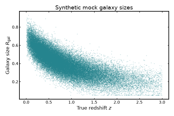
Synthetic mock catalog#
For demonstration purposes we construct a simple mock galaxy sample with redshifts, magnitudes, and intrinsic sizes.
The galaxy-size distribution is chosen such that high-redshift galaxies are typically smaller on the sky, making them more susceptible to PSF selection effects.
import cmasher as cmr
import matplotlib.pyplot as plt
import numpy as np
from matplotlib.colors import to_rgba

rng = np.random.default_rng(42)

n_gal = 50000

z_true = rng.gamma(shape=2.0, scale=0.45, size=n_gal)
z_true = z_true[(z_true >= 0.0) & (z_true <= 3.0)]

mag = 22.0 + 2.1 * z_true + rng.normal(
    0.0,
    0.4,
    size=z_true.size,
)

r_gal = (
    0.7 / (1.0 + z_true)
    + rng.normal(0.0, 0.08, size=z_true.size)
)
r_gal = np.clip(r_gal, 0.05, None)

color = cmr.take_cmap_colors(
    "viridis",
    1,
    cmap_range=(0.45, 0.45),
    return_fmt="hex",
)[0]

fig, ax = plt.subplots(figsize=(7.5, 5.0))

ax.scatter(
    z_true,
    r_gal,
    s=6,
    color=to_rgba(color, 0.25),
    edgecolors="none",
)

ax.set_xlabel(r"True redshift $z$")
ax.set_ylabel(r"Galaxy size $R_{\rm gal}$")
ax.set_title("Synthetic mock galaxy sizes")

plt.tight_layout()
(Source code, png, hires.png, pdf)

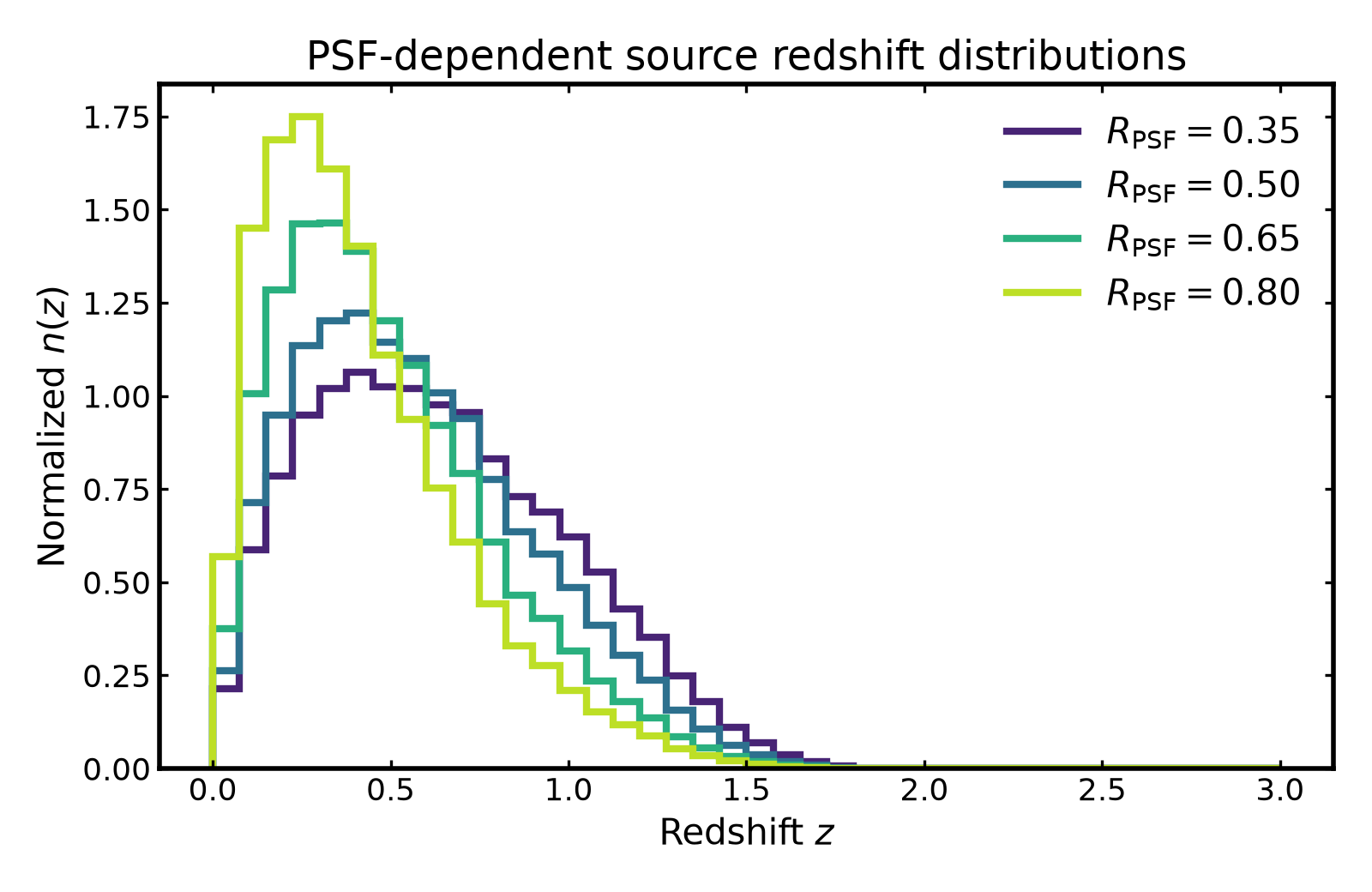
PSF-dependent redshift distributions#
Increasing the PSF size changes the weighted source sample. In this synthetic example, larger PSFs preferentially remove smaller galaxies, which changes the normalized redshift distribution.
import cmasher as cmr
import matplotlib.pyplot as plt
import numpy as np

from binny import NZTomography

rng = np.random.default_rng(42)

n_gal = 50000

z_true = rng.gamma(shape=2.0, scale=0.45, size=n_gal)
z_true = z_true[(z_true >= 0.0) & (z_true <= 3.0)]

mag = 22.0 + 2.1 * z_true + rng.normal(
    0.0,
    0.4,
    size=z_true.size,
)

r_gal = (
    0.7 / (1.0 + z_true)
    + rng.normal(0.0, 0.08, size=z_true.size)
)
r_gal = np.clip(r_gal, 0.05, None)

maglim = 25.0
r_psf_values = np.array([0.35, 0.50, 0.65, 0.80])
z_edges = np.linspace(0.0, 3.0, 41)

result = NZTomography.calibrate_psf_depth_from_mock(
    z_true=z_true,
    mag=mag,
    r_gal=r_gal,
    maglims=np.array([maglim]),
    r_psf_values=r_psf_values,
    area_deg2=100.0,
    z_edges=z_edges,
    selection_kind="sigmoid",
    normalize_nz=True,
)

colors = cmr.take_cmap_colors(
    "viridis",
    len(r_psf_values),
    cmap_range=(0.1, 0.9),
    return_fmt="hex",
)

fig, ax = plt.subplots(figsize=(8.0, 5.2))

for color, row in zip(colors, result["results"], strict=True):
    if np.isclose(row["maglim"], maglim):
        ax.stairs(
            row["nz"],
            z_edges,
            color=color,
            linewidth=3.0,
            label=rf"$R_{{\rm PSF}}={row['r_psf']:.2f}$",
        )

ax.set_xlabel(r"Redshift $z$")
ax.set_ylabel(r"Normalized $n(z)$")
ax.set_title(r"PSF-dependent source redshift distributions")
ax.legend(frameon=False)

plt.tight_layout()
(Source code, png, hires.png, pdf)

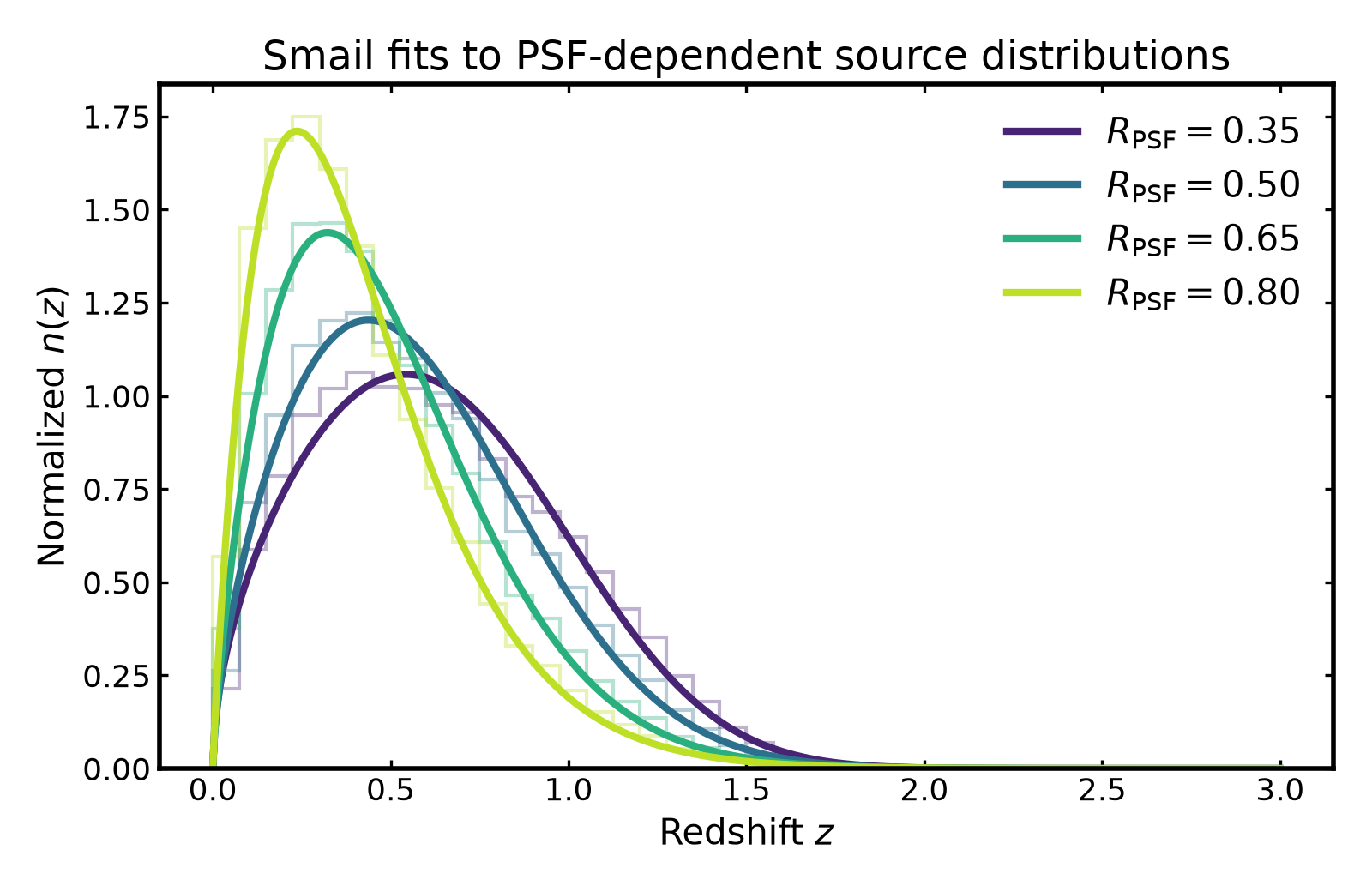
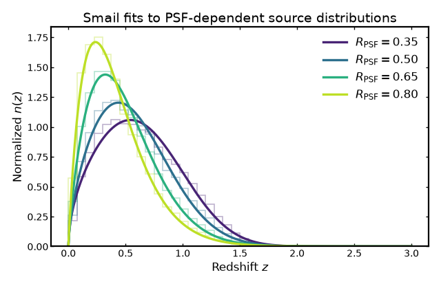
Smail fits to PSF-dependent redshift distributions#
The calibrated PSF-dependent samples can also be compressed into smooth analytic Smail distributions. This is useful when a forecast needs a compact parametric representation of the PSF-dependent source sample.
import cmasher as cmr
import matplotlib.pyplot as plt
import numpy as np

from binny import NZTomography

rng = np.random.default_rng(42)

n_gal = 50000

z_true = rng.gamma(shape=2.0, scale=0.45, size=n_gal)
z_true = z_true[(z_true >= 0.0) & (z_true <= 3.0)]

mag = 22.0 + 2.1 * z_true + rng.normal(
    0.0,
    0.4,
    size=z_true.size,
)

r_gal = (
    0.7 / (1.0 + z_true)
    + rng.normal(0.0, 0.08, size=z_true.size)
)
r_gal = np.clip(r_gal, 0.05, None)

maglim = 25.0
r_psf_values = np.array([0.35, 0.50, 0.65, 0.80])
z_edges = np.linspace(0.0, 3.0, 41)

result = NZTomography.calibrate_psf_depth_from_mock(
    z_true=z_true,
    mag=mag,
    r_gal=r_gal,
    maglims=np.array([maglim]),
    r_psf_values=r_psf_values,
    area_deg2=100.0,
    z_edges=z_edges,
    selection_kind="sigmoid",
    normalize_nz=True,
)

colors = cmr.take_cmap_colors(
    "viridis",
    len(r_psf_values),
    cmap_range=(0.1, 0.9),
    return_fmt="hex",
)

z_fine = np.linspace(0.0, 3.0, 600)

fig, ax = plt.subplots(figsize=(8.0, 5.2))

for color, row in zip(colors, result["results"], strict=True):
    if not np.isclose(row["maglim"], maglim):
        continue

    smail_result = NZTomography.fit_smail_from_mock(
        row["z"],
        weights=row["weights"],
        z_max=3.0,
    )

    if not smail_result["ok"]:
        continue

    params = smail_result["params"]

    nz_fit = NZTomography.nz_model(
        "smail",
        z_fine,
        z0=params["z0"],
        alpha=params["alpha"],
        beta=params["beta"],
        normalize=True,
    )

    ax.stairs(
        row["nz"],
        z_edges,
        color=color,
        linewidth=1.5,
        alpha=0.35,
    )

    ax.plot(
        z_fine,
        nz_fit,
        color=color,
        lw=3.0,
        label=rf"$R_{{\rm PSF}}={row['r_psf']:.2f}$",
    )

ax.set_xlabel(r"Redshift $z$")
ax.set_ylabel(r"Normalized $n(z)$")
ax.set_title(r"Smail fits to PSF-dependent source distributions")
ax.legend(frameon=False)

plt.tight_layout()
(Source code, png, hires.png, pdf)
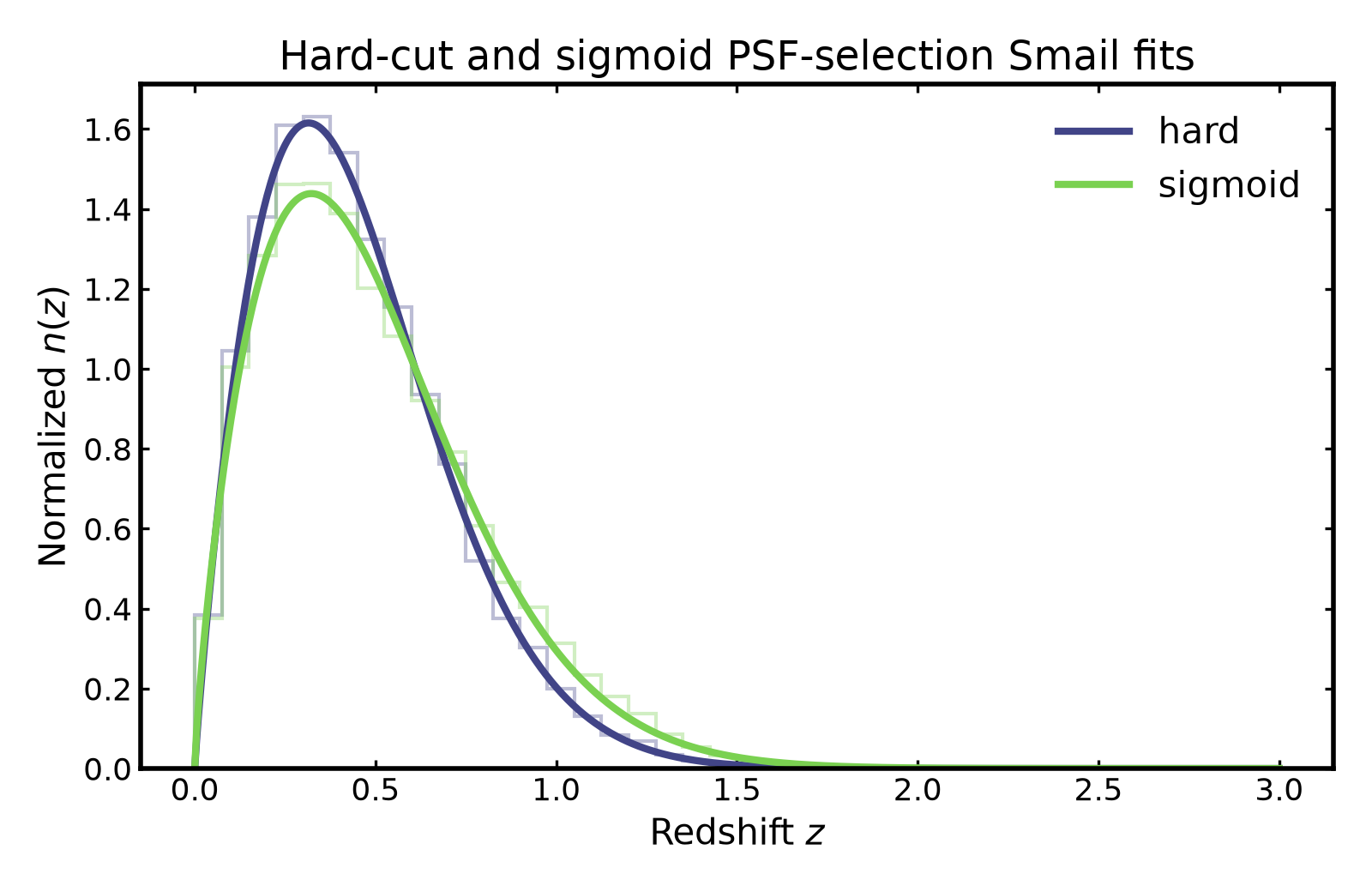
Hard-cut versus sigmoid Smail fits#
The choice of PSF-selection model can also be propagated into the fitted Smail representation. A hard cut gives a binary selected sample, while the sigmoid model keeps the same galaxies with continuous shear-selection weights. This comparison shows how both assumptions change the calibrated redshift distribution and its smooth Smail fit.
import cmasher as cmr
import matplotlib.pyplot as plt
import numpy as np

from binny import NZTomography

rng = np.random.default_rng(42)

n_gal = 50000

z_true = rng.gamma(shape=2.0, scale=0.45, size=n_gal)
z_true = z_true[(z_true >= 0.0) & (z_true <= 3.0)]

mag = 22.0 + 2.1 * z_true + rng.normal(
    0.0,
    0.4,
    size=z_true.size,
)

r_gal = (
    0.7 / (1.0 + z_true)
    + rng.normal(0.0, 0.08, size=z_true.size)
)
r_gal = np.clip(r_gal, 0.05, None)

maglim = 25.0
r_psf = 0.65
z_edges = np.linspace(0.0, 3.0, 41)
z_fine = np.linspace(0.0, 3.0, 600)

colors = cmr.take_cmap_colors(
    "viridis",
    2,
    cmap_range=(0.2, 0.8),
    return_fmt="hex",
)

fig, ax = plt.subplots(figsize=(8.0, 5.2))

for color, selection_kind in zip(colors, ["hard", "sigmoid"], strict=True):
    result = NZTomography.calibrate_psf_depth_from_mock(
        z_true=z_true,
        mag=mag,
        r_gal=r_gal,
        maglims=np.array([maglim]),
        r_psf_values=np.array([r_psf]),
        area_deg2=100.0,
        z_edges=z_edges,
        selection_kind=selection_kind,
        normalize_nz=True,
    )

    row = result["results"][0]

    smail_result = NZTomography.fit_smail_from_mock(
        row["z"],
        weights=row["weights"],
        z_max=3.0,
    )

    if not smail_result["ok"]:
        continue

    params = smail_result["params"]

    nz_fit = NZTomography.nz_model(
        "smail",
        z_fine,
        z0=params["z0"],
        alpha=params["alpha"],
        beta=params["beta"],
        normalize=True,
    )

    ax.stairs(
        row["nz"],
        z_edges,
        color=color,
        linewidth=1.5,
        alpha=0.35,
    )

    ax.plot(
        z_fine,
        nz_fit,
        color=color,
        lw=3.0,
        label=selection_kind,
    )

ax.set_xlabel(r"Redshift $z$")
ax.set_ylabel(r"Normalized $n(z)$")
ax.set_title(r"Hard-cut and sigmoid PSF-selection Smail fits")
ax.legend(frameon=False)

plt.tight_layout()
(Source code, png, hires.png, pdf)
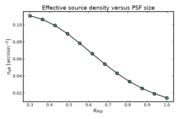
Effective source density#
The same calibration also returns the effective source density for each combination of limiting magnitude and PSF size.
For a fixed limiting magnitude, the effective source density decreases as the PSF becomes larger.
import cmasher as cmr
import matplotlib.pyplot as plt
import numpy as np
from matplotlib.colors import to_rgba

from binny import NZTomography

rng = np.random.default_rng(42)

n_gal = 50000

z_true = rng.gamma(shape=2.0, scale=0.45, size=n_gal)
z_true = z_true[(z_true >= 0.0) & (z_true <= 3.0)]

mag = 22.0 + 2.1 * z_true + rng.normal(
    0.0,
    0.4,
    size=z_true.size,
)

r_gal = (
    0.7 / (1.0 + z_true)
    + rng.normal(0.0, 0.08, size=z_true.size)
)
r_gal = np.clip(r_gal, 0.05, None)

maglim = 25.0
r_psf_values = np.linspace(0.3, 1.0, 12)
z_edges = np.linspace(0.0, 3.0, 41)

result = NZTomography.calibrate_psf_depth_from_mock(
    z_true=z_true,
    mag=mag,
    r_gal=r_gal,
    maglims=np.array([maglim]),
    r_psf_values=r_psf_values,
    area_deg2=100.0,
    z_edges=z_edges,
    selection_kind="sigmoid",
    normalize_nz=True,
)

psf = []
neff = []

for row in result["results"]:
    if np.isclose(row["maglim"], maglim):
        psf.append(row["r_psf"])
        neff.append(row["neff_arcmin2"])

color = cmr.take_cmap_colors(
    "viridis",
    1,
    cmap_range=(0.65, 0.65),
    return_fmt="hex",
)[0]

fig, ax = plt.subplots(figsize=(7.5, 5.0))

ax.plot(
    psf,
    neff,
    color="k",
    lw=2.0,
    zorder=1,
)
ax.scatter(
    psf,
    neff,
    s=70,
    color=to_rgba(color, 0.65),
    edgecolor="k",
    linewidth=2.0,
    zorder=2,
)

ax.set_xlabel(r"$R_{\rm PSF}$")
ax.set_ylabel(r"$n_{\rm eff}$ [arcmin$^{-2}$]")
ax.set_title(r"Effective source density versus PSF size")

plt.tight_layout()
(Source code, png, hires.png, pdf)
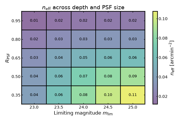
Joint depth–PSF selection grid#
The calibration can also be evaluated across both limiting magnitude and PSF size. This gives a compact grid describing how image quality and survey depth jointly affect the usable weak-lensing source sample.
import matplotlib.pyplot as plt
import numpy as np
from matplotlib.colors import ListedColormap

from binny import NZTomography

rng = np.random.default_rng(42)

n_gal = 50000

z_true = rng.gamma(shape=2.0, scale=0.45, size=n_gal)
z_true = z_true[(z_true >= 0.0) & (z_true <= 3.0)]

mag = 22.0 + 2.1 * z_true + rng.normal(
    0.0,
    0.4,
    size=z_true.size,
)

r_gal = (
    0.7 / (1.0 + z_true)
    + rng.normal(0.0, 0.08, size=z_true.size)
)
r_gal = np.clip(r_gal, 0.05, None)

maglims = np.array([23.0, 23.5, 24.0, 24.5, 25.0])
r_psf_values = np.array([0.35, 0.50, 0.65, 0.80, 0.95])
z_edges = np.linspace(0.0, 3.0, 41)

result = NZTomography.calibrate_psf_depth_from_mock(
    z_true=z_true,
    mag=mag,
    r_gal=r_gal,
    maglims=maglims,
    r_psf_values=r_psf_values,
    area_deg2=100.0,
    z_edges=z_edges,
    selection_kind="sigmoid",
    normalize_nz=True,
)

grid = np.full(
    (len(r_psf_values), len(maglims)),
    np.nan,
)

for row in result["results"]:
    i = np.where(np.isclose(r_psf_values, row["r_psf"]))[0][0]
    j = np.where(np.isclose(maglims, row["maglim"]))[0][0]
    grid[i, j] = row["neff_arcmin2"]

base = plt.get_cmap("viridis")
colors = base(np.linspace(0.05, 0.95, 256))
colors[:, -1] = 0.6
cmap_transparent = ListedColormap(colors)

fig, ax = plt.subplots(figsize=(7.8, 5.2))

im = ax.imshow(
    grid,
    origin="lower",
    aspect="auto",
    cmap=cmap_transparent,
    interpolation="none",
)

n_rows, n_cols = grid.shape

ax.set_xticks(np.arange(n_cols))
ax.set_yticks(np.arange(n_rows))
ax.set_xticklabels([f"{m:.1f}" for m in maglims])
ax.set_yticklabels([f"{r:.2f}" for r in r_psf_values])

ax.set_xticks(np.arange(-0.5, n_cols, 1), minor=True)
ax.set_yticks(np.arange(-0.5, n_rows, 1), minor=True)
ax.grid(which="minor", color="k", linestyle="-", linewidth=2)
ax.tick_params(which="minor", bottom=False, left=False)

for i in range(n_rows):
    for j in range(n_cols):
        ax.text(
            j,
            i,
            f"{grid[i, j]:.2f}",
            ha="center",
            va="center",
            fontsize=12,
            color="k",
        )

ax.set_xlabel(r"Limiting magnitude $m_{\rm lim}$")
ax.set_ylabel(r"$R_{\rm PSF}$")
ax.set_title(r"$n_{\rm eff}$ across depth and PSF size")

plt.colorbar(
    im,
    ax=ax,
    label=r"$n_{\rm eff}$ [arcmin$^{-2}$]",
)

plt.tight_layout()
(Source code, png, hires.png, pdf)

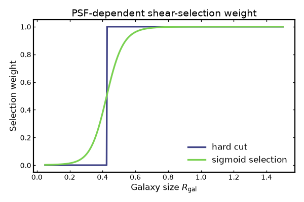
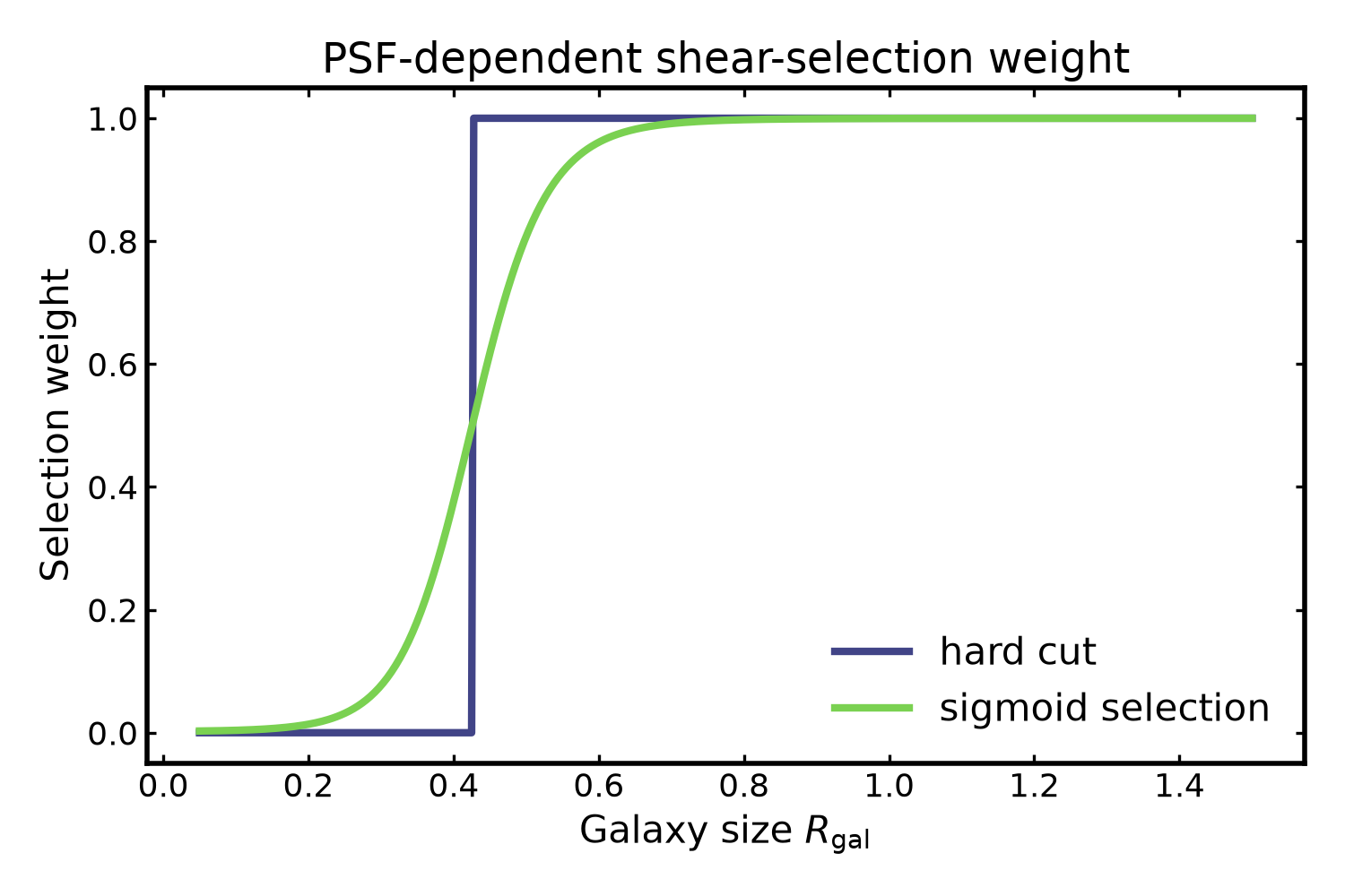
Smooth PSF selection weights#
The PSF-dependent selection can be modelled either as a hard resolution cut or as a smooth sigmoid transition.
The hard cut keeps or removes galaxies abruptly once their resolution factor crosses the selection threshold. The sigmoid model instead assigns continuous weights between zero and one, giving a smoother approximation to how shear measurement efficiency changes as galaxies become less resolved relative to the PSF.
import cmasher as cmr
import matplotlib.pyplot as plt
import numpy as np

from binny.nz.psf_selection import shear_selection_weight

r_gal = np.linspace(0.05, 1.5, 500)
r_psf = 0.65

hard = shear_selection_weight(
    r_gal,
    r_psf=r_psf,
    r_min=0.3,
    kind="hard",
)

sigmoid = shear_selection_weight(
    r_gal,
    r_psf=r_psf,
    r_min=0.3,
    kind="sigmoid",
    width=0.05,
)

colors = cmr.take_cmap_colors(
    "viridis",
    2,
    cmap_range=(0.2, 0.8),
    return_fmt="hex",
)

fig, ax = plt.subplots(figsize=(7.5, 5.0))

ax.plot(
    r_gal,
    hard,
    color=colors[0],
    lw=3,
    ls="-",
    label="hard cut",
)

ax.plot(
    r_gal,
    sigmoid,
    color=colors[1],
    lw=3.0,
    label="sigmoid selection",
)

ax.set_xlabel(r"Galaxy size $R_{\rm gal}$")
ax.set_ylabel("Selection weight")
ax.set_title(r"PSF-dependent shear-selection weight")
ax.legend(frameon=False)

plt.tight_layout()
(Source code, png, hires.png, pdf)

Notes#
Increasing PSF size preferentially removes compact galaxies.
This can change both \(n_{\rm eff}\) and the source redshift distribution.
The effect can depend on survey depth because deeper samples contain fainter and often smaller galaxies.
The calibration is useful for propagating image-quality assumptions into weak-lensing forecasts.