Sample composition

Binny can combine several tomographic samples into one logical sample collection. This is useful when different galaxy samples should contribute to one parent redshift distribution, while still preserving sample-aware bin labels for downstream selections and data-vector construction.

There are two common use cases:

• physically adding samples together, for example when LRG and ELG should be treated as one effective lens population;

• keeping samples separate but using sample-aware labels, for example when a data vector must distinguish ("LRG", 0) from ("ELG", 0).

The first case uses combine_parent_nz or combine_tomography_bins. The second case uses sample_bin_labels, sample_bins, and sample_combinations.

This example uses the DESI survey preset and combines the DESI LRG and ELG lens samples.

Combining DESI parent samples

Parent-sample composition adds the parent redshift distributions. If samples are defined on different redshift grids, interpolate=True maps them onto a common grid before summing. By default, the first sample grid is used as the target grid unless z_target is provided explicitly.

from binny import NZTomography


lrg_tomo = NZTomography()
elg_tomo = NZTomography()

lrg = lrg_tomo.build_survey_bins(
    "desi",
    role="lens",
    sample="lrg",
    overrides={"bins": {"edges": [0.4, 0.6, 0.8, 1.0]}},
)

elg = elg_tomo.build_survey_bins(
    "desi",
    role="lens",
    sample="elg",
    overrides={"bins": {"edges": [0.6, 0.9, 1.2, 1.5]}},
)

z_combined, nz_combined = NZTomography.combine_parent_nz(
    [
        {"z": lrg.z, "nz": lrg.nz},
        {"z": elg.z, "nz": elg.nz},
    ],
    interpolate=True,
)

The returned arrays are plain NumPy arrays. This makes the combined parent distribution easy to inspect, plot, or pass into another custom binning step.

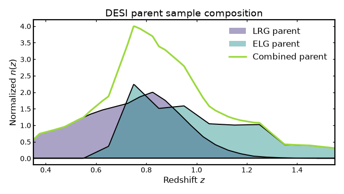
Visualizing parent sample composition

The figure below compares the DESI LRG and ELG parent redshift distributions with their combined parent distribution.

(Source code, png, hires.png, pdf)

Parent-level composition is useful for visual checks, but many analyses need the tomographic bins themselves. In that case, matching bin indices can be summed directly. This requires the samples to have the same bin keys. For example, bin 0 in the combined sample is the sum of bin 0 from each input sample.

Combining matching tomographic bins

If different samples use the same number of tomographic bins, their matching bin indices can also be added together.

combined = NZTomography.combine_tomography_bins(
    [lrg, elg],
    interpolate=True,
)

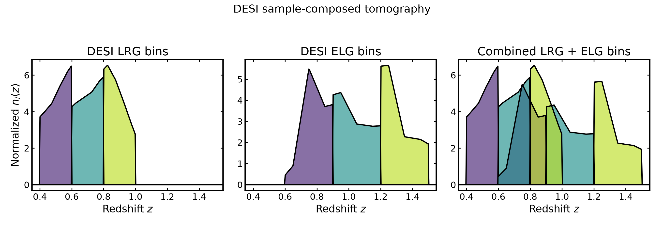
Visualizing combined tomography

The figure below shows the DESI LRG bins, DESI ELG bins, and the combined tomographic sample obtained by summing matching bin indices.

(Source code, png, hires.png, pdf)

Preserving sample-aware bin labels

Sometimes samples should not be summed. Instead, each sample and bin should remain identifiable. This is useful for building sample-aware data vectors.

lenses = {
    "LRG": lrg,
    "ELG": elg,
}

labels = NZTomography.sample_bin_labels(lenses)
bins = NZTomography.sample_bins(lenses)

print(labels)

Building sample-aware combinations

Sample-aware combinations preserve both the sample name and the bin index.

sources = {
    "LSST": lsst_source,
}

lens_source_pairs = NZTomography.sample_combinations(
    lenses,
    sources,
)

print(lens_source_pairs)

For example, if lenses contains DESI LRG and ELG bins, and sources contains LSST source bins, the resulting labels have the form

(("LRG", 0), ("LSST", 0))
(("LRG", 1), ("LSST", 0))
(("ELG", 0), ("LSST", 0))

These labels preserve both the sample identity and tomographic bin index. They can be passed directly to pair-selection routines, covariance builders, forecasting pipelines, or other downstream analyses without losing track of which physical sample each bin originated from.

Summary

Binny supports two complementary approaches for working with multiple tomographic samples:

• combine_parent_nz combines parent redshift distributions;

• combine_tomography_bins combines matching tomographic bins;

• sample_bin_labels and sample_bins flatten multiple samples while preserving sample identities;

• sample_combinations constructs sample-aware combinations across one or more collections.

Together, these utilities make it possible to either merge samples into a single effective population or preserve their identities for analyses that require sample-aware bookkeeping.