 LF-weighted n(z) models#
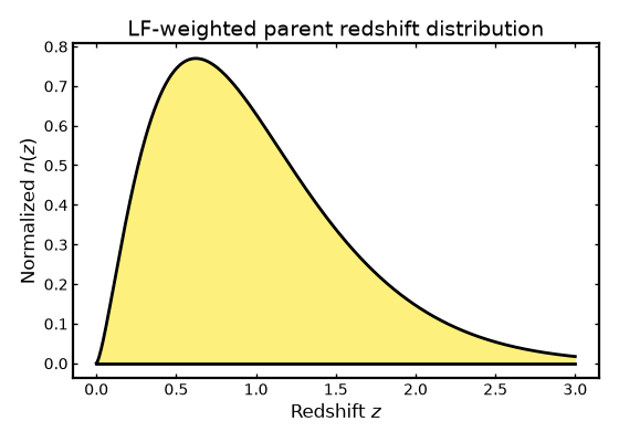
This page provides executable examples showing how to build luminosity function-weighted redshift distributions \(n(z)\) with Binny and LFKit.
The model combines three ingredients:
a redshift grid supplied by
Binny,a
PyCCLcosmology used for distances and volume weights,an
LFKitluminosity function used for the magnitude-limited LF integral.
The resulting parent redshift distribution has the form
where \(M_{\mathrm{lim}}(z)\) is obtained from the apparent magnitude limit and the luminosity distance.
This follows the same basic idea used in luminosity function-based
redshift-distribution modelling for weak-lensing source samples, as in
Šarčević et al. 2025, Joint Modelling of Astrophysical Systematics for
Cosmology with LSST Cosmic Shear (arXiv:2406.03352) and for galaxy clustering samples in
Van Daalen and White 2018 (arXiv:1703.05326).
Basic LF-weighted n(z)#
We begin with the simplest direct call to the registered
"luminosity_function" model. The user supplies a redshift grid,
an LFKit luminosity function object, a PyCCL cosmology, and magnitude-limit
settings. Binny then passes CCL-backed luminosity-distance and volume-weight
helpers into LFKit.
import cmasher as cmr
import matplotlib.pyplot as plt
import numpy as np
import pyccl as ccl

from lfkit import LuminosityFunction
from binny import NZTomography

z = np.linspace(0.0, 3.0, 500)

cosmo = ccl.Cosmology(
    Omega_c=0.2607,
    Omega_b=0.049,
    h=0.6766,
    sigma8=0.8102,
    n_s=0.9665,
    transfer_function="bbks",
    matter_power_spectrum="linear",
)

lf = LuminosityFunction(
    model="schechter",
    parameters={
        "phi_star": 3.0e-3,
        "m_star": -21.0,
        "alpha": -1.25,
    },
)

nz = NZTomography.nz_model(
    "luminosity_function",
    z,
    lf=lf,
    cosmo=cosmo,
    m_lim=25.3,
    m_bright=-26.0,
    n_m=512,
    normalize=True,
)

color = cmr.take_cmap_colors(
    "viridis",
    3,
    cmap_range=(0.0, 1.0),
    return_fmt="hex",
)[-1]

fig, ax = plt.subplots(figsize=(7.0, 5.0))

ax.fill_between(
    z,
    0.0,
    nz,
    color=color,
    alpha=0.6,
    linewidth=0.0,
    zorder=10,
)
ax.plot(z, nz, color="k", linewidth=2.5, zorder=20)
ax.plot(z, np.zeros_like(z), color="k", linewidth=2.5, zorder=100)

ax.set_xlabel("Redshift $z$")
ax.set_ylabel(r"Normalized $n(z)$")
ax.set_title("LF-weighted parent redshift distribution")

plt.tight_layout()
(Source code, png, hires.png, pdf)
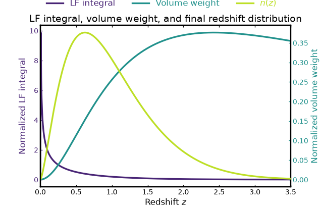
How LF and volume combine#
This example shows the construction more explicitly. The luminosity function integral gives the magnitude-limited galaxy density as a function of redshift. The cosmology supplies the comoving volume weight. Their product gives the unnormalized redshift distribution.
This is a compact version of the usual convolution-style diagnostic plot: LF contribution, survey volume contribution, and final redshift distribution.
import cmasher as cmr
import matplotlib.pyplot as plt
import numpy as np
import pyccl as ccl

from lfkit import LuminosityFunction
from binny.cosmology.ccl_wrappers import (
    comoving_volume_weight,
    luminosity_distance_mpc,
)
from binny import NZTomography

z = np.linspace(0.0, 3.5, 600)

cosmo = ccl.Cosmology(
    Omega_c=0.2607,
    Omega_b=0.049,
    h=0.6766,
    sigma8=0.8102,
    n_s=0.9665,
    transfer_function="bbks",
    matter_power_spectrum="linear",
)

lf = LuminosityFunction(
    model="schechter",
    parameters={
        "phi_star": 3.0e-3,
        "m_star": -21.0,
        "alpha": -1.25,
    },
)

lf_integral = NZTomography.nz_model(
    "luminosity_function",
    z,
    lf=lf,
    cosmo=cosmo,
    m_lim=25.3,
    m_bright=-26.0,
    n_m=512,
    volume_weight_fn=lambda z_eval: np.ones_like(z_eval),
    normalize=True,
)

volume = comoving_volume_weight(cosmo, z)
volume_scaled = volume / np.trapezoid(volume, z)

nz = NZTomography.nz_model(
    "luminosity_function",
    z,
    lf=lf,
    cosmo=cosmo,
    m_lim=25.3,
    m_bright=-26.0,
    n_m=512,
    normalize=True,
)

colors = cmr.take_cmap_colors(
    "viridis",
    5,
    cmap_range=(0.1, 0.9),
    return_fmt="hex",
)

color_lf = colors[0]
color_volume = colors[2]
color_nz = colors[4]

fig, ax1 = plt.subplots(figsize=(8.0, 5.2))
fig.patch.set_facecolor("white")

ax2 = ax1.twinx()
ax3 = ax1.twinx()
ax3.spines["right"].set_position(("outward", 65))

line1, = ax1.plot(
    z,
    lf_integral,
    color=color_lf,
    linewidth=3.0,
    label="LF integral",
)
line2, = ax2.plot(
    z,
    volume_scaled,
    color=color_volume,
    linewidth=3.0,
    label="Volume weight",
)
line3, = ax3.plot(
    z,
    nz,
    color=color_nz,
    linewidth=3.0,
    label=r"$n(z)$",
)

ax1.set_xlabel("Redshift $z$")
ax1.set_ylabel("Normalized LF integral", color=color_lf)
ax2.set_ylabel("Normalized volume weight", color=color_volume)
ax3.set_ylabel(r"Normalized $n(z)$", color=color_nz)

ax1.tick_params(axis="y", colors=color_lf)
ax2.tick_params(axis="y", colors=color_volume)
ax3.tick_params(axis="y", colors=color_nz)

for ax in [ax1, ax2, ax3]:
    ax.tick_params(direction="in", axis="both", which="both")

lines = [line1, line2, line3]
labels = [line.get_label() for line in lines]

legend = fig.legend(
    lines,
    labels,
    frameon=False,
    loc="upper center",
    bbox_to_anchor=(0.5, 1.04),
    ncol=3,
)

for line, text in zip(legend.get_lines(), legend.get_texts(), strict=True):
    text.set_color(line.get_color())

ax1.set_xlim(z.min(), z.max())
ax1.set_title("LF integral, volume weight, and final redshift distribution")
(Source code, png, hires.png, pdf)
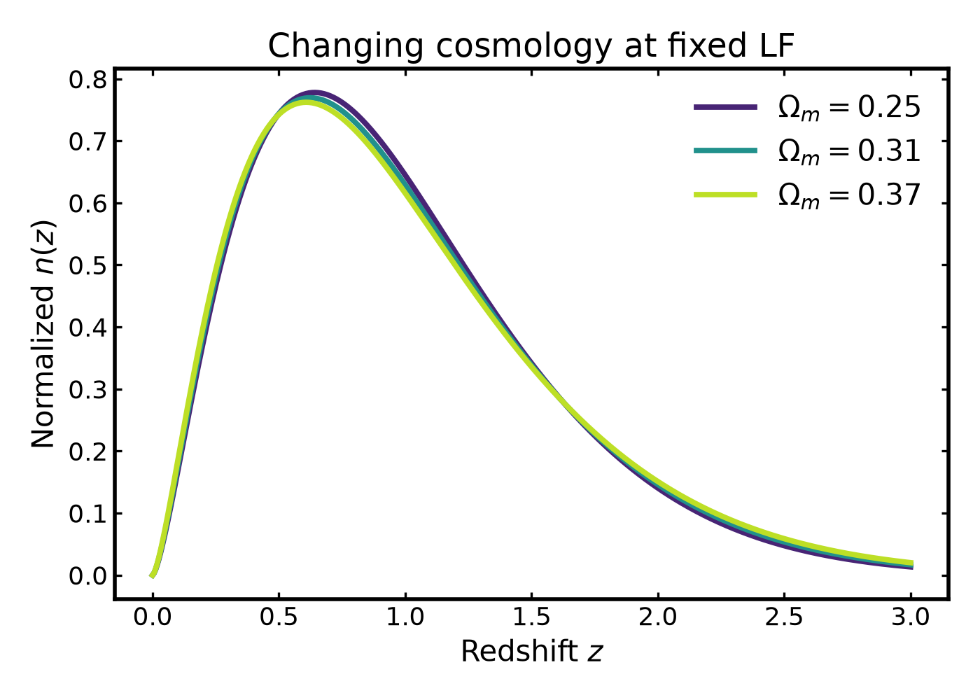
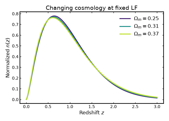
Changing cosmology at fixed LF#
The LF is held fixed here while the cosmology is changed. This isolates the effect of the luminosity distance and comoving volume element on the final magnitude-limited redshift distribution.
import cmasher as cmr
import matplotlib.pyplot as plt
import numpy as np
import pyccl as ccl

from lfkit import LuminosityFunction
from binny import NZTomography

z = np.linspace(0.0, 3.0, 500)

cosmologies = {
    r"$\Omega_m = 0.25$": ccl.Cosmology(
        Omega_c=0.201,
        Omega_b=0.049,
        h=0.6766,
        sigma8=0.8102,
        n_s=0.9665,
        transfer_function="bbks",
        matter_power_spectrum="linear",
    ),
    r"$\Omega_m = 0.31$": ccl.Cosmology(
        Omega_c=0.2607,
        Omega_b=0.049,
        h=0.6766,
        sigma8=0.8102,
        n_s=0.9665,
        transfer_function="bbks",
        matter_power_spectrum="linear",
    ),
    r"$\Omega_m = 0.37$": ccl.Cosmology(
        Omega_c=0.321,
        Omega_b=0.049,
        h=0.6766,
        sigma8=0.8102,
        n_s=0.9665,
        transfer_function="bbks",
        matter_power_spectrum="linear",
    ),
}

lf = LuminosityFunction(
    model="schechter",
    parameters={
        "phi_star": 3.0e-3,
        "m_star": -21.0,
        "alpha": -1.25,
    },
)

colors = cmr.take_cmap_colors(
    "viridis",
    len(cosmologies),
    cmap_range=(0.1, 0.9),
    return_fmt="hex",
)

fig, ax = plt.subplots(figsize=(7.0, 5.0))

for (label, cosmo), color in zip(cosmologies.items(), colors, strict=True):
    nz = NZTomography.nz_model(
        "luminosity_function",
        z,
        lf=lf,
        cosmo=cosmo,
        m_lim=25.3,
        m_bright=-26.0,
        n_m=512,
        normalize=True,
    )

    ax.plot(
        z,
        nz,
        color=color,
        linewidth=2.8,
        label=label,
    )

ax.set_xlabel("Redshift $z$")
ax.set_ylabel(r"Normalized $n(z)$")
ax.set_title("Changing cosmology at fixed LF")
ax.legend(frameon=False, loc="best")

plt.tight_layout()
(Source code, png, hires.png, pdf)
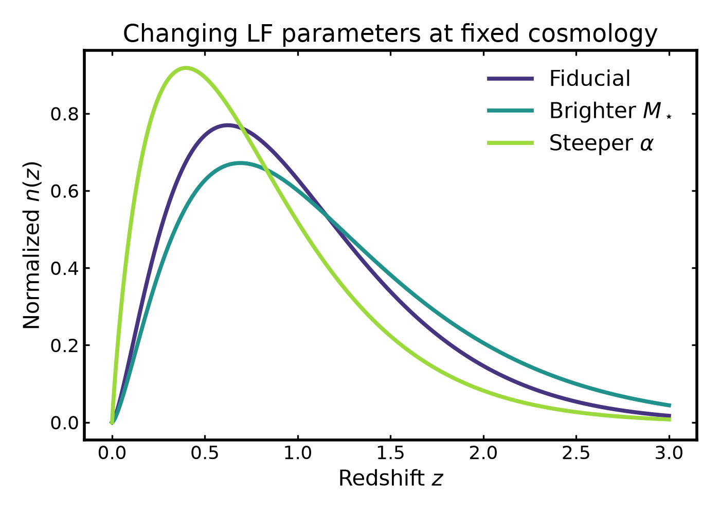
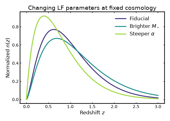
Changing LF at fixed cosmology#
Now the cosmology is fixed and the LF parameters are changed. This isolates how the assumed luminosity function shape affects the magnitude-limited parent redshift distribution.
import cmasher as cmr
import matplotlib.pyplot as plt
import numpy as np
import pyccl as ccl

from lfkit import LuminosityFunction
from binny import NZTomography

z = np.linspace(0.0, 3.0, 500)

cosmo = ccl.Cosmology(
    Omega_c=0.2607,
    Omega_b=0.049,
    h=0.6766,
    sigma8=0.8102,
    n_s=0.9665,
    transfer_function="bbks",
    matter_power_spectrum="linear",
)

luminosity_functions = {
    r"Fiducial": LuminosityFunction(
        model="schechter",
        parameters={
            "phi_star": 3.0e-3,
            "m_star": -21.0,
            "alpha": -1.25,
        },
    ),
    r"Brighter $M_\star$": LuminosityFunction(
        model="schechter",
        parameters={
            "phi_star": 3.0e-3,
            "m_star": -21.6,
            "alpha": -1.25,
        },
    ),
    r"Steeper $\alpha$": LuminosityFunction(
        model="schechter",
        parameters={
            "phi_star": 3.0e-3,
            "m_star": -21.0,
            "alpha": -1.55,
        },
    ),
}

colors = cmr.take_cmap_colors(
    "viridis",
    len(luminosity_functions),
    cmap_range=(0.15, 0.85),
    return_fmt="hex",
)

fig, ax = plt.subplots(figsize=(7.0, 5.0))

for (label, lf), color in zip(luminosity_functions.items(), colors, strict=True):
    nz = NZTomography.nz_model(
        "luminosity_function",
        z,
        lf=lf,
        cosmo=cosmo,
        m_lim=25.3,
        m_bright=-26.0,
        n_m=512,
        normalize=True,
    )

    ax.plot(
        z,
        nz,
        color=color,
        linewidth=2.8,
        label=label,
    )

ax.set_xlabel("Redshift $z$")
ax.set_ylabel(r"Normalized $n(z)$")
ax.set_title("Changing LF parameters at fixed cosmology")
ax.legend(frameon=False, loc="best")

plt.tight_layout()
(Source code, png, hires.png, pdf)
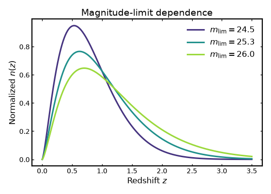
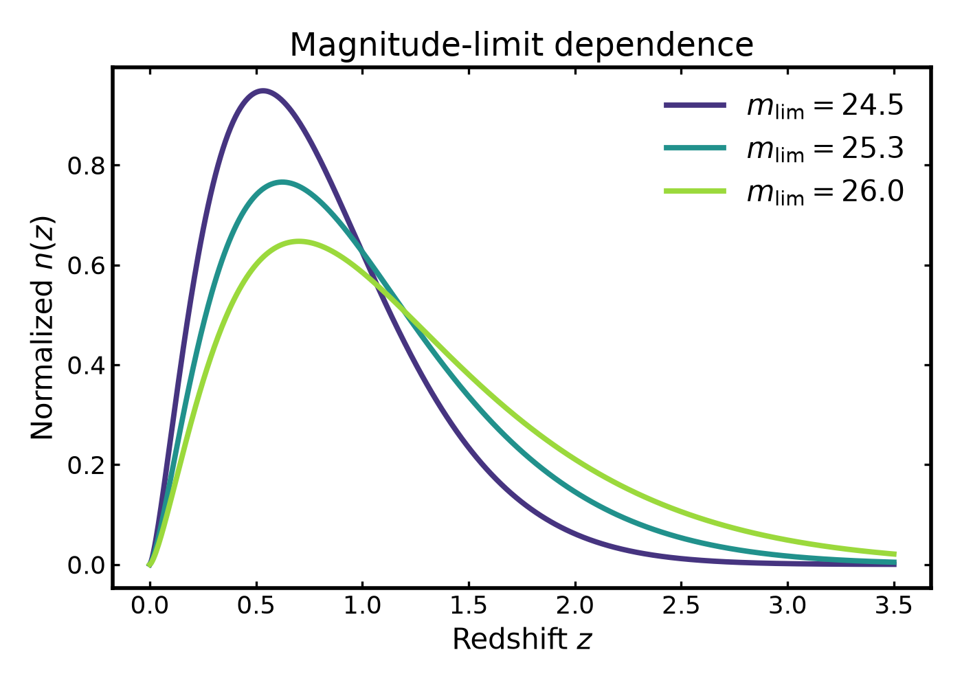
Magnitude-limit dependence#
The apparent magnitude limit controls how faint the observed sample can be. For a fixed LF and cosmology, deeper magnitude limits include more faint galaxies and usually push the redshift distribution toward larger redshift.
import cmasher as cmr
import matplotlib.pyplot as plt
import numpy as np
import pyccl as ccl

from lfkit import LuminosityFunction
from binny import NZTomography

z = np.linspace(0.0, 3.5, 600)

cosmo = ccl.Cosmology(
    Omega_c=0.2607,
    Omega_b=0.049,
    h=0.6766,
    sigma8=0.8102,
    n_s=0.9665,
    transfer_function="bbks",
    matter_power_spectrum="linear",
)

lf = LuminosityFunction(
    model="schechter",
    parameters={
        "phi_star": 3.0e-3,
        "m_star": -21.0,
        "alpha": -1.25,
    },
)

magnitude_limits = [24.5, 25.3, 26.0]

colors = cmr.take_cmap_colors(
    "viridis",
    len(magnitude_limits),
    cmap_range=(0.15, 0.85),
    return_fmt="hex",
)

fig, ax = plt.subplots(figsize=(7.0, 5.0))

for m_lim, color in zip(magnitude_limits, colors, strict=True):
    nz = NZTomography.nz_model(
        "luminosity_function",
        z,
        lf=lf,
        cosmo=cosmo,
        m_lim=m_lim,
        m_bright=-26.0,
        n_m=512,
        normalize=True,
    )

    ax.plot(
        z,
        nz,
        color=color,
        linewidth=2.8,
        label=rf"$m_{{\rm lim}} = {m_lim:.1f}$",
    )

ax.set_xlabel("Redshift $z$")
ax.set_ylabel(r"Normalized $n(z)$")
ax.set_title("Magnitude-limit dependence")
ax.legend(frameon=False, loc="best")

plt.tight_layout()
(Source code, png, hires.png, pdf)

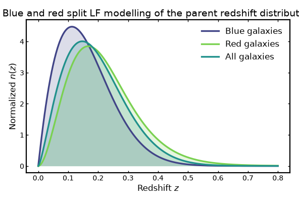
GAMA blue and red split modelling#
This example shows how the underlying parent \(n(z)\) can be modelled from separate luminosity functions for blue, red and all (full sample) galaxies. We use the GAMA (Loveday et al. arXiv:1111.0166) r-band blue and red galaxy fits and evolve the Schechter parameters with the GAMA :math:`Q and \(P\) evolution model.
import cmasher as cmr
import matplotlib.pyplot as plt
import numpy as np
import pyccl as ccl

from lfkit import LuminosityFunction
from binny import NZTomography

def gama_lfkit_evolving_schechter(
    absolute_mag,
    z,
    *,
    phi_star,
    m_star,
    alpha,
    q,
    p,
    z0=0.1,
):
    absolute_mag = np.asarray(absolute_mag)
    z = np.asarray(z)

    if absolute_mag.ndim > z.ndim:
        z = z[..., None]

    lf = LuminosityFunction.schechter(
        phi_star=phi_star * 10.0 ** (0.4 * p * z),
        m_star=m_star - q * (z - z0),
        alpha=alpha,
    )

    return lf.phi(absolute_mag)

z = np.linspace(0.0, 0.8, 500)

cosmo = ccl.Cosmology(
    Omega_c=0.2607,
    Omega_b=0.049,
    h=0.6766,
    sigma8=0.8102,
    n_s=0.9665,
    transfer_function="bbks",
    matter_power_spectrum="linear",
)

nz_blue = NZTomography.nz_model(
    "luminosity_function",
    z,
    lf=gama_lfkit_evolving_schechter,
    cosmo=cosmo,
    m_lim=19.8,
    m_bright=-24.0,
    n_m=512,
    normalize=True,
    phi_star=0.0038,
    m_star=-20.45,
    alpha=-1.49,
    q=0.8,
    p=2.9,
)

nz_red = NZTomography.nz_model(
    "luminosity_function",
    z,
    lf=gama_lfkit_evolving_schechter,
    cosmo=cosmo,
    m_lim=19.8,
    m_bright=-24.0,
    n_m=512,
    normalize=True,
    phi_star=0.0111,
    m_star=-20.34,
    alpha=-0.57,
    q=1.8,
    p=-1.2,
)

nz_all = NZTomography.nz_model(
    "luminosity_function",
    z,
    lf=gama_lfkit_evolving_schechter,
    cosmo=cosmo,
    m_lim=19.8,
    m_bright=-24.0,
    n_m=512,
    normalize=True,
    phi_star=0.94,
    m_star=-20.7,
    alpha=-1.23,
    q=0.7,
    p=1.8,
)

colors = cmr.take_cmap_colors(
    "viridis",
    3,
    cmap_range=(0.2, 0.8),
    return_fmt="hex",
)

fig, ax = plt.subplots(figsize=(7.4, 5.0))

ax.plot(z, nz_blue, color=colors[0], linewidth=3.0, label="Blue galaxies")
ax.fill_between(z, 0.0, nz_blue, color=colors[0], alpha=0.18, linewidth=0.0)

ax.plot(z, nz_red, color=colors[2], linewidth=3.0, label="Red galaxies")
ax.fill_between(z, 0.0, nz_red, color=colors[2], alpha=0.18, linewidth=0.0)

ax.plot(z, nz_all, color=colors[1], linewidth=3.0, label="All galaxies")
ax.fill_between(z, 0.0, nz_all, color=colors[1], alpha=0.18, linewidth=0.0)

ax.set_xlabel("Redshift $z$")
ax.set_ylabel(r"Normalized $n(z)$")
ax.set_title("Blue and red split LF modelling of the parent redshift distribution")
ax.legend(frameon=False, loc="best")

plt.tight_layout()
(Source code, png, hires.png, pdf)
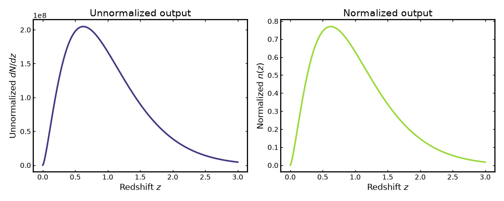
Normalized versus unnormalized output#
For tomography, the normalized parent \(n(z)\) is usually what you want. For diagnostics, the unnormalized curve is also useful because it preserves the change in total number density caused by the LF, cosmology, or magnitude limit.
import cmasher as cmr
import matplotlib.pyplot as plt
import numpy as np
import pyccl as ccl

from lfkit import LuminosityFunction
from binny import NZTomography

z = np.linspace(0.0, 3.0, 500)

cosmo = ccl.Cosmology(
    Omega_c=0.2607,
    Omega_b=0.049,
    h=0.6766,
    sigma8=0.8102,
    n_s=0.9665,
    transfer_function="bbks",
    matter_power_spectrum="linear",
)

lf = LuminosityFunction(
    model="schechter",
    parameters={
        "phi_star": 3.0e-3,
        "m_star": -21.0,
        "alpha": -1.25,
    },
)

nz_unnormalized = NZTomography.nz_model(
    "luminosity_function",
    z,
    lf=lf,
    cosmo=cosmo,
    m_lim=25.3,
    m_bright=-26.0,
    n_m=512,
    normalize=False,
)

nz_normalized = NZTomography.nz_model(
    "luminosity_function",
    z,
    lf=lf,
    cosmo=cosmo,
    m_lim=25.3,
    m_bright=-26.0,
    n_m=512,
    normalize=True,
)

colors = cmr.take_cmap_colors(
    "viridis",
    2,
    cmap_range=(0.15, 0.85),
    return_fmt="hex",
)

fig, axes = plt.subplots(1, 2, figsize=(12.5, 5.0))

axes[0].plot(
    z,
    nz_unnormalized,
    color=colors[0],
    linewidth=2.8,
)
axes[0].set_xlabel("Redshift $z$")
axes[0].set_ylabel(r"Unnormalized $dN/dz$")
axes[0].set_title("Unnormalized output")
axes[0].ticklabel_format(style="sci", axis="y", scilimits=(0, 0))

axes[1].plot(
    z,
    nz_normalized,
    color=colors[1],
    linewidth=2.8,
)
axes[1].set_xlabel("Redshift $z$")
axes[1].set_ylabel(r"Normalized $n(z)$")
axes[1].set_title("Normalized output")

plt.tight_layout()
(Source code, png, hires.png, pdf)
Inspecting returned values#
The returned object is a NumPy array evaluated on the supplied redshift grid. This makes it easy to pass into later tomography steps.
import numpy as np
import pyccl as ccl

from lfkit import LuminosityFunction
from binny import NZTomography

z = np.linspace(0.0, 3.0, 500)

cosmo = ccl.Cosmology(
    Omega_c=0.2607,
    Omega_b=0.049,
    h=0.6766,
    sigma8=0.8102,
    n_s=0.9665,
    transfer_function="bbks",
    matter_power_spectrum="linear",
)

lf = LuminosityFunction(
    model="schechter",
    parameters={
        "phi_star": 3.0e-3,
        "m_star": -21.0,
        "alpha": -1.25,
    },
)

nz = NZTomography.nz_model(
    "luminosity_function",
    z,
    lf=lf,
    cosmo=cosmo,
    m_lim=25.3,
    m_bright=-26.0,
    n_m=512,
    normalize=True,
)

print("z grid:")
print(z)
print()
print("LF-weighted n(z):")
print(nz)
print()
print("Shape:", nz.shape)
print("All non-negative:", bool(np.all(nz >= 0.0)))
print("Integral:", float(np.trapezoid(nz, z)))
Notes#
The LF physics and magnitude-limit integration live in LFKit.
Binny supplies the redshift grid and CCL-backed distance and volume helpers.
Setting
normalize=Truemakes the returned parent distribution integrate to unity over the supplied redshift grid.Setting
normalize=Falseis useful when checking number-density changes.The output is a parent \(n(z)\), not a set of tomographic bins. To build tomography from this distribution, pass the evaluated parent curve into the usual Binny tomography workflow.